

Advanced Concepts of Probability & Statistics for AI Engineers
A complete, CTO-authored guide from first principles to enterprise-scale decision systems — the discipline that turns raw data into calibrated, trustworthy AI.
Curriculum Map
- 01 Executive Summary — The Decision Engine of AI
- 02 Populations, Sampling & Descriptive Statistics
- 03 Variance & Covariance
- 04 Random Variables & Probability Foundations
- 05 Common Probability Distributions
- 06 The Central Limit Theorem
- 07 Conditional Probability & Bayes’ Theorem
- 08 Maximum Likelihood Estimation
- 09 Linear & Logistic Regression
- 10 Hypothesis Testing & Confidence Intervals
- 11 A/B Testing at Enterprise Scale
- 12 Statistics Inside Modern AI & LLMs
- 13 Real-World Industry Applications
- 14 Best Practices & Conclusion
Why Statistics Is the Decision Engine of AI in 2026
Every model that review with engineering teams inside global telecom and technology organizations eventually reduces to the same question: how confident are we in this number, and what would it take to be wrong? That question is statistics, not machine learning — and the engineers who can answer it rigorously are the ones whose systems survive contact with production traffic instead of quietly degrading in ways nobody notices for months.
Linear algebra gives a model its shape; statistics gives it its judgment. Every loss function is a statistical estimator in disguise, every training run is a sampling process from an unknown data-generating distribution, and every “the model says 87% confidence” claim is either a calibrated probability grounded in real statistical theory — or a number that looks like one but isn’t. In 2026, with AI systems making autonomous decisions across telecom networks, financial pipelines, and customer-facing products, the gap between those two cases is where outages, biased outcomes, and eroded trust come from.
Where Statistics Actually Shows Up in Your Stack
Loss Functions
Cross-entropy, MSE, and every common loss are maximum likelihood estimators wearing a different name.
Experimentation
A/B tests, hypothesis testing, and confidence intervals decide what actually ships to production.
Uncertainty Quantification
Calibrated confidence scores and Bayesian methods separate trustworthy predictions from confident guesses.
Sampling & Bias
Every training set is a sample — understanding sampling bias is how you predict where a model will fail.
By the end of this guide you will be able to reason fluently about sampling and estimation, choose and interpret the right probability distribution for a problem, apply Bayes’ theorem to update beliefs with evidence, understand loss functions as maximum likelihood estimators, run and interpret statistically valid A/B tests, and connect all of this to how modern AI systems quantify — and sometimes fail to quantify — their own uncertainty.
Populations, Sampling & Descriptive Statistics
A population is every possible unit you could observe — every user, every network packet, every transaction that has ever occurred or ever will. A sample is the finite subset you actually collect. Nearly every statistical error in production AI systems traces back to treating a biased or unrepresentative sample as if it faithfully described the full population.
Three Measures of Center — and Why They Disagree
| Measure | Definition | Sensitive to Outliers? | Best Used When |
|---|---|---|---|
| Mean | Sum divided by count | Yes — heavily | Symmetric, outlier-free distributions |
| Median | Middle value when sorted | No — robust | Skewed data: income, latency, revenue |
| Mode | Most frequent value | No | Categorical data, multimodal distributions |
A single dashboard reporting only the mean latency of an API is a classic production trap: a handful of extreme outliers can drag the mean far from what a typical user actually experiences, while the median — and better still, the 95th or 99th percentile — tells the real story engineers need for SLAs.
Expected value generalizes the mean from “the average of what I observed” to “the average of what I would observe if I could sample the process infinitely.” This distinction matters enormously in AI: a model’s expected reward in reinforcement learning, or the expected loss a training objective minimizes, are both statements about an idealized infinite population, not the finite batch actually seen during one training step.
Sampling Methods — How You Choose Matters as Much as How Much
Not all samples are created equal, and the method used to select one determines whether the statistics computed from it generalize to the population at all. Simple random sampling gives every unit an equal chance of selection and is the theoretical gold standard, but it’s rarely how real production data actually arrives. Stratified sampling deliberately samples within known subgroups — by region, device type, or customer tier — to guarantee every important segment is represented proportionally, which matters enormously for a telecom operator training a model that must perform consistently across urban and rural network conditions. Convenience sampling — using whatever data happens to be easiest to collect, such as only logged-in users or only users on a particular app version — is the single most common source of silent bias in production machine learning pipelines, because it feels like “real data” while systematically excluding entire populations the model will eventually be asked to serve.
This is why a model trained on last quarter’s most active users can quietly fail on new signups: the training sample was never a random draw from the population the model is now being asked to generalize to. Auditing the sampling process that produced a training set is, in practice, one of the highest-leverage and most frequently skipped steps in a machine learning pipeline.
Variance & Covariance
If the mean answers “where is the data centered?”, variance answers “how spread out is it?” — and covariance answers “do two variables move together?” These three quantities, taken together, are the entire foundation of everything from feature scaling to PCA to portfolio risk models.
Variance
Average squared distance from the mean — the mathematical definition of “how noisy is this.”
Standard Deviation
The square root of variance, expressed in the original units — far more interpretable for reporting.
Positive Covariance
Two variables tend to rise and fall together — e.g. ad spend and impressions.
Negative Covariance
One rises as the other falls — e.g. churn rate and customer satisfaction.
The Covariance Matrix — the Bridge to Linear Algebra
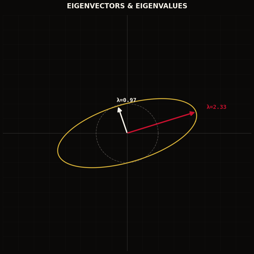
Stack the pairwise covariances of every feature in a dataset into a matrix and you get the covariance matrix — the exact object whose eigendecomposition produces Principal Component Analysis. This is the concrete link between the statistics in this guide and the linear algebra covered in the companion guide in this series: PCA is nothing more than “find the directions of maximum variance,” expressed with matrix machinery.
Feature scaling — standardizing every input to zero mean and unit variance before training — exists precisely because gradient-based optimizers converge far more reliably when every feature’s variance is on a comparable scale; a single high-variance feature can otherwise dominate the loss landscape and destabilize training.
Random Variables & Probability Foundations
A random variable is a function that assigns a numeric value to the outcome of an uncertain process — a customer’s next click, a packet’s latency, a token sampled from a language model’s output distribution. Every random variable is one of two fundamental types, and confusing them is a common source of modeling errors.
| Type | Definition | AI Example |
|---|---|---|
| Discrete | Takes countable, distinct values | Class label, number of retries, token ID |
| Continuous | Takes any value in a range | Latency in milliseconds, model confidence score, sensor reading |
Three Rules That Govern All Probability
- Non-negativity — every probability is between 0 and 1, inclusive.
- Normalization — probabilities of all possible outcomes sum (or integrate) to exactly 1.
- Additivity — the probability of mutually exclusive events is the sum of their individual probabilities.
These three rules are precisely what a softmax layer enforces on a model’s raw output logits — converting arbitrary real numbers into a valid probability distribution over classes. Every time you see a softmax, you’re watching an engineered enforcement of the three axioms of probability.
Common Probability Distributions
A probability distribution is a model of a data-generating process. Choosing the right one — or recognizing which one your data actually follows — is one of the highest-leverage skills in applied statistics.
| Distribution | Shape | AI / Telecom Use Case |
|---|---|---|
| Normal (Gaussian) | Symmetric bell curve | Measurement noise, weight initialization, model residuals |
| Binomial | Discrete, bounded trials | Conversion counts, A/B test success rates, packet-loss events |
| Uniform | Flat, equal probability | Random initialization ranges, dropout masks, hashing |
| Poisson | Discrete, unbounded, rate-based | Requests per second, call arrivals, network events per interval |
| Exponential | Continuous, memoryless decay | Time between network failures, session duration modeling |
The Central Limit Theorem
The Central Limit Theorem (CLT) is arguably the single most consequential result in applied statistics: the distribution of a sample mean approaches a normal distribution as sample size grows, regardless of the shape of the underlying population distribution.
This single theorem is why confidence intervals, standard errors, and p-values built on normal-distribution assumptions remain valid for A/B tests and telemetry aggregation even when the raw underlying data — response times, revenue per user, error rates — is wildly non-normal. It’s also why increasing sample size is the most reliable lever for shrinking uncertainty: the standard error of a sample mean shrinks proportionally to 1/√n.
Conditional Probability & Bayes’ Theorem
Conditional probability — the probability of an event given that another has occurred — is how every recommendation engine, spam filter, and diagnostic model reasons under partial information. Bayes’ theorem is the formal rule for updating a belief when new evidence arrives, and it is arguably the most economically important eight-word idea in applied statistics.
Why Engineers Get Bayes’ Theorem Wrong in Production
The classic failure mode is ignoring the base rate. A fraud model with 99% accuracy sounds excellent — until you account for the fact that genuine fraud might occur in only 0.1% of transactions, meaning the vast majority of “fraud” flags from an imperfect classifier are false positives. Bayes’ theorem forces this base-rate reasoning explicitly, which is exactly why it is the correct framework for spam filtering, medical-style diagnostic AI, and any fraud or anomaly system where the event of interest is rare.
| Term | Meaning | Production Example |
|---|---|---|
| Prior | Belief before seeing evidence | Base fraud rate across all transactions |
| Likelihood | How probable the evidence is, given the hypothesis | How often fraud produces this transaction pattern |
| Posterior | Updated belief after evidence | Probability this specific transaction is fraud |
Maximum Likelihood Estimation
Maximum Likelihood Estimation (MLE) answers a deceptively simple question: given the data I observed, what parameter values make that data most probable? This isn’t a niche statistical technique — it is, quite literally, what training a model means.
Loss Functions Are MLE in Disguise
Mean Squared Error
MSE is exactly the MLE solution when you assume Gaussian-distributed residuals around the model’s predictions.
Cross-Entropy
Cross-entropy loss is exactly the MLE solution under a categorical (softmax) output distribution.
Next-Token Prediction
Training an LLM on next-token prediction is MLE over a categorical distribution across the vocabulary.
Why This Matters
Understanding a loss function’s MLE assumptions tells you exactly when it will fail — e.g. MSE under heavy-tailed noise.
Linear & Logistic Regression
Regression is where statistics and machine learning fully merge: both are fitting a parametric model to data by maximizing likelihood — the difference between “classical statistics” and “machine learning” here is mostly a difference of vocabulary and scale, not of underlying mathematics.
| Linear Regression | Logistic Regression | |
|---|---|---|
| Predicts | A continuous value | A probability between 0 and 1 |
| Output function | y = Wx + b | σ(Wx + b), sigmoid-squashed |
| Assumed noise model | Gaussian residuals | Bernoulli / categorical outcome |
| Loss function | Mean squared error | Cross-entropy (log loss) |
| Typical use | Forecasting revenue, latency, demand | Churn prediction, fraud flagging, click-through |
# Logistic regression, the workhorse baseline for binary classification
from sklearn.linear_model import LogisticRegression

model = LogisticRegression()
model.fit(X_train, y_train)
probabilities = model.predict_proba(X_test)[:, 1]  # calibrated probability of class 1
Regularization — A Statistical Prior in Disguise
L1 (Lasso) and L2 (Ridge) regularization, ubiquitous across both classical regression and deep learning, have a clean statistical interpretation that’s easy to lose sight of in day-to-day engineering: they are exactly equivalent to placing a Bayesian prior on the model’s weights and finding the maximum a posteriori (MAP) estimate rather than the plain maximum likelihood estimate. L2 regularization corresponds to a Gaussian prior centered at zero, which is why it shrinks weights smoothly toward zero without forcing them there. L1 regularization corresponds to a Laplace prior, whose sharper peak at zero is exactly why it tends to produce genuinely sparse solutions — driving entire coefficients to exactly zero rather than merely shrinking them. Recognizing regularization as “adding statistical prior knowledge to the estimation problem” turns a hyperparameter you tune by grid search into a modeling decision you can reason about directly: how strongly do I believe, before seeing any data, that most features shouldn’t matter?
Hypothesis Testing & Confidence Intervals
Hypothesis testing is the formal framework for asking “is this observed effect real, or could it plausibly be explained by random chance alone?” Every production experimentation platform is, underneath its dashboard, running this exact logic.
- State the null hypothesis (H₀) — the assumption of “no effect,” e.g. “the new checkout flow converts at the same rate as the old one.”
- Choose a significance level (α) — typically 0.05, the false-positive rate you’re willing to accept.
- Collect data and compute a test statistic — how far the observed result sits from what H₀ predicts, in standard-error units.
- Compute the p-value — the probability of seeing a result this extreme (or more) if H₀ were actually true.
- Decide — if p < α, reject H₀ in favor of the alternative; otherwise, you have not found sufficient evidence of an effect.
Confidence Intervals — A Range, Not a Point
A 95% confidence interval means: if we repeated this sampling process many times, 95% of the intervals constructed this way would contain the true population parameter. It does not mean “there’s a 95% chance the true value is in this specific interval” — a common and consequential misinterpretation. Reporting a range instead of a single point estimate is what separates a defensible business decision from a false sense of precision.
A/B Testing at Enterprise Scale
At a global telecom or technology company running thousands of simultaneous experiments, A/B testing stops being a spreadsheet exercise and becomes an infrastructure problem — one built directly on the statistical foundations in this guide.
Four Problems That Only Appear at Enterprise Scale
Multiple Comparisons
Running hundreds of simultaneous tests inflates false-positive rates — correction methods like Bonferroni or FDR control become mandatory.
Peeking Bias
Checking results repeatedly before a test concludes invalidates the p-value — sequential testing methods exist specifically to fix this.
Network Effects
Users in a social or telecom network aren’t independent samples — a treatment can leak across the control group.
Novelty & Seasonality
Short experiments can be misled by novelty effects or day-of-week seasonality — run duration must account for a full cycle.
Sample Size Planning — The Step Most Teams Skip
Before launching any experiment, a power analysis answers a question far too many teams skip until it’s too late: given the expected effect size, the baseline conversion rate, and the desired statistical power (conventionally 80%), how many users does this test actually need to reach a trustworthy conclusion? Under-powered experiments are one of the most expensive silent failures in enterprise product development — a test that runs for two weeks and shows “no significant difference” is frequently not evidence of no effect at all, but evidence that the sample size was never large enough to detect the effect size that mattered. Running a power calculation before launch, not after a disappointing result, is what separates a genuinely inconclusive experiment from a bad one dressed up as a null result.
Statistics Inside Modern AI & LLMs
Every large language model is, at inference time, sampling from a learned probability distribution over the next token — temperature, top-k, and top-p sampling are all direct manipulations of that distribution’s shape.
| Sampling Control | Statistical Effect |
|---|---|
| Temperature | Rescales the distribution — higher temperature flattens it toward uniform, increasing randomness |
| Top-k | Truncates the distribution to the k most probable tokens before sampling |
| Top-p (nucleus) | Truncates to the smallest set of tokens whose cumulative probability exceeds p |
Calibration — Does “80% Confident” Actually Mean 80%?
A model is well-calibrated if, among all predictions it makes at 80% confidence, roughly 80% actually turn out correct. Modern large neural networks are frequently overconfident by default — a critical concern for any AI system in telecom, finance, or healthcare where a confidence score informs a real downstream decision. Calibration techniques — temperature scaling, Platt scaling, conformal prediction — exist specifically to correct this gap between a model’s stated and actual reliability.
Real-World Industry Applications
Telecom Network Reliability
Call-drop and packet-loss events are modeled as Poisson and binomial processes respectively, letting engineering teams set statistically grounded SLA thresholds instead of arbitrary ones, and flag true anomalies rather than normal statistical variation.
Fraud & Risk Scoring
Bayesian base-rate reasoning (Chapter 7) combined with logistic regression remains the backbone of interpretable, auditable fraud-scoring systems — a regulatory requirement in many financial and telecom billing contexts where a black-box score alone isn’t defensible.
Demand Forecasting & Capacity Planning
Confidence intervals around demand forecasts — not just point predictions — are what let network capacity planners size infrastructure investments against a defensible worst-case, not just an expected-case number.
Customer Experience & Experimentation
Every UI change, pricing test, and retention campaign at scale runs through the A/B testing infrastructure from Chapter 11 — statistically invalid experiments are one of the most expensive, hardest-to-detect sources of wasted product investment in any large organization.
Best Practices & Conclusion
Five Statistical Habits Every AI Engineer Should Build
- Never report a mean without context. Pair it with a median, a standard deviation, or a percentile — a single number without spread hides risk.
- Distrust round numbers of confidence. If a model reports “95% confident” verify whether that number is actually calibrated, not just a softmax output.
- Pre-register your hypothesis. Decide what you’re testing and your significance threshold before looking at the data — not after, when peeking bias creeps in.
- Account for multiple comparisons. Testing many metrics or many variants simultaneously requires a correction, or you will find “significant” results in pure noise.
- Ask what distribution a loss function assumes. Every loss function is a statistical bet about your data’s noise model — know what bet you’re making.
Probability and statistics are what let an AI system reason honestly about the world instead of just pattern-matching against it. The organizations pulling ahead in 2026 are the ones whose engineers can move fluidly between a loss function’s statistical assumptions, an experiment’s p-value, and a model’s calibrated confidence — treating all three as expressions of the same discipline, not three unrelated skills. That fluency is what turns a model that merely predicts into a system an enterprise can actually trust to decide.
Appendix A.1 — Formula Quick Reference
| Concept | Formula |
|---|---|
| Expected value | E[X] = Σ x·P(x) |
| Variance | Var(X) = E[(X−μ)²] |
| Bayes’ theorem | P(A|B) = P(B|A)·P(A) / P(B) |
| Standard error | SE = σ / √n |
| MLE objective | argmax P(data | θ) |
| Logistic function | σ(z) = 1 / (1 + e⁻ᶻ) |
Appendix A.2 — Production Readiness Checklist
- Summary statistics reported with spread, not just a single mean
- Model confidence scores checked for calibration, not assumed accurate
- A/B tests pre-registered with a defined hypothesis and significance level
- Multiple-comparison correction applied when testing several metrics or variants
- Sample size and expected run time calculated before launching an experiment
- Loss function’s distributional assumptions understood and validated against data
- Confidence intervals reported alongside every point forecast used for planning
- Sampling process audited for representativeness before training on any dataset
Go Build Systems That Know What They Don’t Know 📊
This guide is part of EDUNXT Tech Learning’s ongoing series translating core engineering concepts into practical, actionable frameworks for global founders and engineering teams.
Restart the Curriculum