

Advanced Concepts of Calculus: A Complete Guide from Fundamentals to Enterprise-Level for AI Engineers in 2026
Every model you ship, every optimizer you tune, and every production incident you debug in a large-scale AI system traces back to five calculus ideas. This is the guide I give every engineering team before they touch a training pipeline.

// contents
- Why Calculus Still Decides Who Wins in AI (2026)
- 01 — Derivatives & Gradients
- 02 — The Gradient Descent Algorithm
- 03 — Vector & Matrix Calculus: Jacobian and Hessian
- 04 — The Chain Rule and Backpropagation
- 05 — Fundamentals of Optimization
- 06 — Calculus at Enterprise Scale: Telecom & Global AI
- The 2026 Learning Roadmap (SOP)
- AI & ML Education Series
Why Calculus Still Decides Who Wins in AI in 2026
Walk into any serious AI engineering org in 2026 — a hyperscaler, a telecom operator standing up its own foundation models for network intelligence, or a mid-size product team fine-tuning open-weight models — and you will find the same quiet truth. The engineers who can reason about why a model trains, diverges, or plateaus are the ones who get promoted into architecture roles. The rest stay dependent on frameworks they cannot debug. Calculus is the difference.
This is not a nostalgia trip back to university lecture halls. The calculus that matters for a production AI engineer today is narrower and more practical than a full undergraduate syllabus, but it is non-negotiable. It shows up the moment your loss curve does something you did not expect: a training run that stalls at a plateau, a fine-tune that explodes into NaNs, a recommender system whose gradients vanish across forty layers, a telecom traffic-forecasting model whose optimizer keeps bouncing between two states instead of converging. In every one of these cases, the fix is calculus, not luck.
This guide provides training to new engineering hires at a global technology and telecom company: as a complete, self-contained reference that takes you from the fundamentals — derivatives and gradients — through to the enterprise-level reasoning you need when you are optimizing models across distributed GPU clusters and live network infrastructure. Treat it as both a presentation and a standing operating document. Bookmark it, print it, hand it to your next hire.
Derivatives & Gradients
The single measurement every learning algorithm is built on.
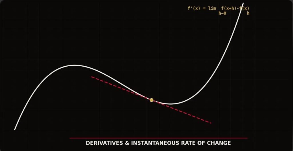
A derivative answers one question: if I nudge this input by an infinitesimally small amount, how much does the output change, and in which direction? That is the entire concept. Formally, for a function f(x), the derivative at a point is:
In machine learning, we almost never work with a single-variable function. A model might have 7 billion parameters, and the “output” we care about is a single scalar: the loss. The derivative of a multivariable function with respect to each of its inputs, collected into a vector, is the gradient:
This one object — the gradient — is the entire engine of modern AI training. It tells every parameter in your network, simultaneously, which direction to move to increase (or, with a sign flip, decrease) the loss. Everything downstream — optimizers, learning-rate schedules, regularization, even hardware design decisions like why GPUs are built around matrix-multiply throughput — exists to compute and apply this vector efficiently, billions of times per training run.
Partial derivatives
Hold every variable constant except one, and differentiate with respect to that one. This is how you build up a gradient one coordinate at a time, and it is the operation autodiff frameworks like PyTorch and JAX perform under the hood, millions of times per second, across a computational graph.
Directional derivatives
The rate of change of a function along an arbitrary direction, not just along an axis. Directional derivatives explain why gradient descent moves diagonally across a loss surface instead of one axis at a time — it always follows the steepest available direction.
Why does this matter at the enterprise level? Because every cost you are optimizing in production — model accuracy, inference latency, energy draw per training epoch, even a telecom operator’s network-congestion score — can be expressed as a differentiable (or approximately differentiable) function. If it is differentiable, it is learnable. Recognizing which business metrics can be turned into a differentiable loss function is, itself, a core AI engineering skill, and it starts with understanding what a derivative actually represents.
The Gradient Descent Algorithm
How a vector of derivatives becomes a trained model.
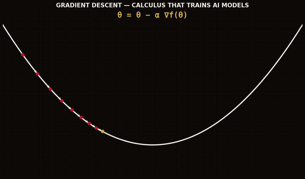
Gradient descent takes the gradient from Section 01 and uses it to iteratively update parameters so the loss goes down. The update rule is deceptively simple:
Because the gradient points toward steepest ascent, subtracting it moves you toward steepest descent — downhill on the loss surface. The learning rate, η, controls the size of each step. Set it too high and the optimizer overshoots and oscillates or diverges; set it too low and training crawls, or gets trapped in a shallow region of the loss surface for far longer than your compute budget allows.

The three regimes: batch, stochastic, and mini-batch
In practice you never compute the gradient over your entire dataset at once except in small academic examples. Enterprise-scale training operates in one of three regimes, and choosing correctly is a genuine architecture decision, not a hyperparameter afterthought.
| Variant | Gradient computed over | Where it’s used in production |
|---|---|---|
| Batch gradient descent | Entire dataset per step | Small, well-understood convex problems; rarely used at scale |
| Stochastic gradient descent (SGD) | One example per step | Online learning, streaming telecom event data, edge fine-tuning |
| Mini-batch gradient descent | A batch (e.g. 32–4096 examples) | The default for nearly all deep learning training today |
Modern optimizers: what they actually change
Every optimizer you will touch in 2026 — Adam, AdamW, Lion, Sophia, Muon — is gradient descent with a modification to how the step is computed. Understanding the base algorithm means you can read an optimizer’s update rule and immediately know what problem it is solving.
- Momentum accumulates a running average of past gradients so the optimizer keeps moving through noisy or shallow regions instead of stalling, the same way a ball rolling downhill carries speed through small bumps.
- RMSProp / Adagrad scale the learning rate per-parameter based on the recent magnitude of that parameter’s gradients, so sparse or rarely-updated parameters (common in large embedding tables) still learn efficiently.
- Adam / AdamW combine momentum and per-parameter scaling, which is why it remains the default optimizer for the majority of transformer training in 2026, especially during fine-tuning of large language and multimodal models.
- Second-order and quasi-second-order optimizers (covered fully in Section 03) use curvature information — not just the gradient — to take smarter, better-scaled steps, at the cost of more compute per step.

Vector & Matrix Calculus: The Jacobian and the Hessian
Scaling derivatives from one output to millions, and from slope to curvature.
A single gradient tells you how one scalar loss changes with respect to many parameters. But real systems rarely have just one output. A transformer’s output layer produces a probability distribution over an entire vocabulary; a computer-vision model outputs a full segmentation map; a telecom forecasting model outputs predicted load across every cell in a region, simultaneously. To differentiate a vector-valued function with respect to a vector of inputs, you need the Jacobian.
The Jacobian is the object that autodiff engines are actually built around. When PyTorch or JAX computes backward(), it is efficiently computing Jacobian-vector products layer by layer, without ever materializing the full Jacobian matrix — which, for a large model, would be computationally impossible to store. Understanding the Jacobian is what lets an engineer reason about why certain architectures (very deep networks, recurrent models) are more numerically unstable to train than others: instability is a Jacobian conditioning problem.
The Hessian: measuring curvature, not just slope
The gradient tells you the slope of the loss surface at a point. It says nothing about whether that slope is about to flatten out, steepen, or curve away in a different direction. That second-order information — curvature — comes from the Hessian, the matrix of second partial derivatives:
The Hessian is expensive — for a model with n parameters it is an n × n matrix, which is why almost no one computes the full Hessian for a billion-parameter model. Instead, enterprise training pipelines use Hessian-free and quasi-Newton methods (L-BFGS, K-FAC, Shampoo, and Sophia in 2026’s toolkit) that approximate curvature cheaply, giving many of the convergence benefits of second-order optimization without the full computational cost.
Why curvature matters
Two points can have the same gradient magnitude but wildly different curvature. A first-order optimizer treats them identically and can badly overshoot or undershoot. A curvature-aware optimizer adjusts its step size based on how sharply the loss surface bends, converging faster on ill-conditioned problems.
Eigenvalues of the Hessian
The sign of the Hessian’s eigenvalues at a critical point tells you what kind of point you have found: all positive means a local minimum, all negative means a local maximum, and mixed signs mean a saddle point — the single most important diagnostic in Section 05.
The Chain Rule
The single equation that makes backpropagation possible.
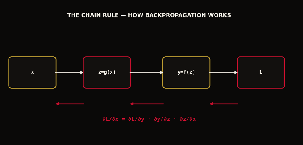
Every neural network is a composition of functions: input goes through a linear layer, then an activation, then another linear layer, then another activation, and so on, dozens or hundreds of times in a modern architecture. To train the network, you need the derivative of the final loss with respect to every single weight buried inside that composition. The chain rule is what makes this tractable:
Extended to a full network, this becomes a product of many local derivatives, one per layer, chained together from the loss all the way back to the very first weight. This is, precisely, backpropagation: not a separate algorithm to memorize, but the chain rule applied systematically across a computational graph, with each layer’s local Jacobian multiplied into the running product as the error signal flows backward.

Why this explains vanishing and exploding gradients
Because backpropagation is a long product of derivatives, its behavior is dictated by simple arithmetic: multiply many numbers smaller than 1 together, and the product shrinks toward zero — the vanishing gradient problem that made very deep networks untrainable before architectural fixes existed. Multiply many numbers larger than 1, and the product explodes — the exploding gradient problem that causes NaN losses and training crashes.
This single insight explains an entire generation of architecture design: residual connections (ResNets, and by extension the residual stream in transformers) exist specifically to give gradients a path with a derivative of exactly 1, so the chain-rule product does not decay across depth. Gradient clipping exists to cap the product’s magnitude directly. Careful weight initialization schemes exist to keep the per-layer Jacobian’s eigenvalues near 1 from the very first training step. None of these are arbitrary engineering tricks — they are direct, deliberate responses to the mathematics of the chain rule.
Fundamentals of Optimization
Local vs. global minima, saddle points, and convexity — reading the shape of the problem you are actually solving.
Training a model is, formally, solving an optimization problem: find the parameters that minimize a loss function. But not all loss surfaces are the same shape, and the shape determines everything about how hard the problem is, which algorithm will work, and how confident you can be that you’ve actually found a good solution.
Local minima vs. global minima
A local minimum is a point where the loss is lower than every nearby point, but not necessarily the lowest possible loss anywhere. A global minimum is the lowest point across the entire loss surface. In classical optimization theory, getting trapped in a poor local minimum was considered the central danger of gradient-based methods.
In modern deep learning, this fear turns out to be largely misplaced — and understanding why is a genuinely important piece of enterprise-level intuition. In the extremely high-dimensional parameter spaces of large neural networks (millions to billions of dimensions), true local minima that are meaningfully worse than the global minimum are statistically rare. Far more common, and far more dangerous, are saddle points.
Saddle points: the real obstacle at scale
A saddle point is a critical point — where the gradient is zero — that is a minimum along some directions and a maximum along others. Picture the shape of a horse’s saddle or a mountain pass: flat and low if you approach from one side, flat and high if you approach from the other.

The danger of a saddle point is not that the optimizer gets permanently stuck — with enough noise (as in stochastic gradient descent) or momentum, it will eventually escape. The danger is speed: near a saddle point the gradient magnitude shrinks toward zero, so training appears to plateau for a long stretch even though it has not actually converged. Recognizing this pattern in a loss curve — a long, flat plateau followed by a sudden further drop — is one of the most practically useful diagnostic skills an AI engineer can have. It is the Hessian’s mixed-sign eigenvalues from Section 03, made visible in your training logs.
Convexity: why it matters even though deep learning isn’t convex
A function is convex if a straight line drawn between any two points on its surface never dips below the surface itself — informally, if it is bowl-shaped, with exactly one minimum and no saddle points or local traps. Convex optimization is well understood and comes with strong theoretical guarantees: gradient descent on a convex function is guaranteed to find the global minimum.

Deep neural networks are almost never convex. Their loss surfaces are high-dimensional, folded, and full of saddle points, flat regions, and sharp ravines like the one pictured above. And yet convexity remains essential knowledge for an enterprise AI engineer for a very practical reason: many sub-problems inside a larger AI system genuinely are convex — logistic regression heads, ridge and lasso regularization terms, linear layers in isolation, many classical control and resource-allocation formulations used in telecom network optimization. Knowing which parts of your system are convex tells you where you can apply strong theoretical guarantees, and which parts require the empirical, iterative tuning that non-convex deep learning demands.
Calculus at Enterprise Scale: Telecom & Global AI Systems
From a whiteboard derivative to a production system running across thousands of GPUs and network nodes.
Everything above is true at the level of a single equation. At enterprise scale — the scale a global telecom or technology company actually operates at — the same calculus gets stretched across distributed systems, and new engineering concerns emerge directly from it.
Distributed gradient computation
When a model is too large to train on a single device, the gradient computation described in Section 01 is split across hundreds or thousands of accelerators. Data parallelism computes gradients on different data shards in parallel and averages them; this average is only mathematically valid because the gradient of a sum is the sum of the gradients — a direct, load-bearing consequence of the linearity of differentiation. Tensor and pipeline parallelism split the Jacobian computation from Section 03 itself across devices, layer by layer or dimension by dimension. Every distributed training framework you will deploy in 2026 — from Megatron-style tensor parallelism to fully sharded data parallel training — is an engineering answer to the question: how do we compute this one mathematical object, the gradient, when it no longer fits on one machine?
Optimization in telecom network intelligence
For a global telecom operator, calculus-driven optimization is not confined to model training. It runs the network itself:
Radio resource management
Allocating bandwidth, power, and spectrum across cells is a continuous constrained-optimization problem, solved in real time using gradient-based and convex-optimization methods to minimize interference and latency.
Predictive maintenance
Forecasting equipment failure from sensor telemetry uses the same gradient descent and chain-rule machinery from Sections 02 and 04, applied to time-series models trained on maintenance logs.
Traffic & demand forecasting
Non-convex deep forecasting models (Section 05) predict network load days or hours ahead, letting operators pre-allocate capacity before congestion happens rather than reacting to it.
Anomaly & fraud detection
Detecting unusual call or data patterns relies on gradient-trained models whose Jacobian sensitivity (Section 03) determines how robust the detector is to small, adversarial perturbations in input data.
Numerical stability as a production concern
At enterprise scale, calculus stops being a purely mathematical topic and becomes an operational one. Mixed-precision training, gradient checkpointing, and loss scaling all exist to keep the chain-rule product from Section 04 numerically stable when computed in 16-bit or 8-bit floating point across a massive distributed job. An engineer who understands why gradients vanish or explode can diagnose a failed multi-million-dollar training run in minutes by reading the gradient norms in the logs. An engineer who only knows how to call .fit() cannot.
The org chart at every serious AI company quietly separates into two groups: engineers who can read a loss curve and know exactly what mathematical object is misbehaving, and engineers who wait for someone else to tell them. Calculus is what moves you from the second group into the first.
The 2026 Learning Roadmap (SOP)
Use this as a standing operating procedure for onboarding AI engineers, structuring an internal training curriculum, or auditing your own readiness. Each stage builds directly on the sections above.
Master single- and multi-variable derivatives by hand
Before touching autodiff, compute gradients manually for simple functions — linear regression, logistic regression — until the notation in Section 01 feels automatic.
Implement gradient descent from scratch, without a framework
Write batch, stochastic, and mini-batch gradient descent in plain NumPy. Then implement momentum and Adam yourself before relying on a library’s version.
Derive the Jacobian and Hessian for a two-layer network
Work through the matrix calculus of Section 03 by hand for a small network, then verify your derivation numerically against PyTorch’s autograd output.
Reconstruct backpropagation from the chain rule alone
Do not memorize the backprop algorithm — re-derive it from Section 04’s chain rule for a three-layer network, then generalize.
Diagnose real training runs using loss-curve shape
Practice identifying plateaus caused by saddle points, divergence caused by an unstable learning rate, and poor conditioning caused by Hessian eigenvalue spread, using Section 05’s diagnostics.
Scale to a distributed, enterprise-grade training job
Apply Section 06: run a data-parallel training job across multiple devices, monitor gradient norms in production, and connect model optimization to a real business or network metric.
Frequently Asked Questions
Do AI engineers really need calculus if frameworks compute gradients automatically?
Automatic differentiation removes the burden of computing derivatives by hand, but it does not remove the need to understand what those derivatives mean. Frameworks like PyTorch and JAX will happily return a gradient of zero, a gradient of infinity, or a gradient that quietly explodes over the course of training — and in every one of those cases, the framework will not tell you why. Diagnosing the failure requires exactly the calculus covered in this guide: recognizing a saddle point from a plateauing loss curve, recognizing an exploding gradient from the chain rule, or recognizing poor conditioning from Hessian eigenvalues. Autodiff automates the arithmetic; it does not automate the judgment.
How much calculus is actually needed — a full university course, or less?
Less than a full course, but more than a summary. In practice, five topics cover the overwhelming majority of what shows up in production AI work: single- and multi-variable derivatives, the gradient descent update rule and its major variants, Jacobians and Hessians at a working level (you rarely need to compute one by hand at scale, but you must understand what they represent), the chain rule as the mechanism behind backpropagation, and the basic vocabulary of optimization — convexity, local versus global minima, and saddle points. This guide is deliberately scoped to exactly those five areas.
What is the single most common calculus-related mistake AI engineers make?
Misreading a plateauing loss curve. Many engineers assume a flat loss curve means the model has converged and stop training, or assume it means the learning rate is too low and increase it aggressively. Section 05 covers why a plateau is very often a saddle point, not a true minimum, and why patience or a small amount of noise (as in SGD) is frequently the correct response rather than a hyperparameter change.
Why do telecom and other non-“pure AI” companies need this level of calculus training?
Because the same mathematics that trains a language model also runs a telecom operator’s radio resource scheduler, its network anomaly detector, and its traffic forecasting system, as detailed in Section 06. Any organization that runs gradient-based optimization anywhere in its stack — and by 2026, nearly every large technology and telecom company does — benefits from engineers who understand the mathematics well enough to debug it in production, not just call a library function and hope for the best.
Is deep learning optimization convex or non-convex, and does it matter which?
Deep learning loss surfaces are almost always non-convex, full of saddle points and irregular curvature, as shown in Section 05. It matters because non-convex optimization comes with no theoretical guarantee of finding the global minimum — success depends heavily on good initialization, normalization, and an optimizer that can navigate flat regions and curved ravines. Recognizing which parts of a larger system are convex (many regularization terms, linear sub-layers, some classical resource-allocation formulations) versus non-convex (the deep network itself) tells an engineer where theory can be trusted and where empirical tuning is required.
Quick-Reference Glossary
| Term | Plain-language definition |
|---|---|
| Derivative | How much an output changes for a tiny change in an input; the instantaneous rate of change. |
| Gradient | A vector of partial derivatives — one per parameter — pointing in the direction of steepest increase of a function. |
| Gradient descent | An algorithm that repeatedly steps parameters in the negative-gradient direction to minimize a loss function. |
| Learning rate | The size of each gradient-descent step; too large causes divergence, too small causes slow training. |
| Jacobian | A matrix of all first-order partial derivatives of a vector-valued function; generalizes the gradient to multiple outputs. |
| Hessian | A matrix of all second-order partial derivatives; describes the curvature of a loss surface. |
| Chain rule | The rule for differentiating a composition of functions; the mathematical basis of backpropagation. |
| Local minimum | A point lower than all nearby points, but not necessarily the lowest point overall. |
| Global minimum | The lowest point across the entire loss surface. |
| Saddle point | A critical point that is a minimum in some directions and a maximum in others; the primary obstacle in high-dimensional training. |
| Convexity | A bowl-shaped function with a single minimum and strong optimization guarantees; deep learning is mostly non-convex. |
| Vanishing/exploding gradients | When the chain-rule product across many layers shrinks toward zero or grows without bound, stalling or destabilizing training. |
Closing Notes from the CTO Desk
None of this calculus is optional trivia for AI engineers building systems in 2026. It is the shared language that connects a whiteboard derivation to a training run, a training run to a production incident, and a production incident to a fix that an engineer can explain with confidence rather than guesswork. The teams that internalize Sections 01 through 05 stop treating their optimizers as black boxes. The organizations that apply Section 06 correctly are the ones running AI systems — from foundation models to live telecom networks — that scale predictably instead of breaking mysteriously at the worst possible moment.
Print this guide. Walk your team through it section by section. Then hold them to the roadmap.
Bring this training into your organization
EDUNXT Tech Learning produces professional, research-driven AI & ML, software engineering, and system-design education for founders and engineering teams worldwide. This guide is part of an ongoing series translating core engineering concepts into practical, actionable frameworks for a global audience.
Explore the full training series →