
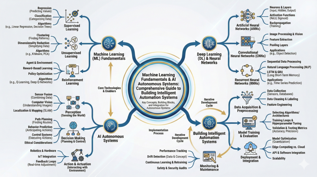
Machine Learning Fundamentals & AI Autonomous Systems : Comprehensive Guide to Building Intelligent Automation Systems
- Executive Summary & The ML Revolution
- Machine Learning Fundamentals
- Core ML Concepts & Algorithms
- Data Pipeline & Preprocessing
- Model Training & Evaluation
- Supervised Learning Systems
- Unsupervised Learning Systems
- Deep Learning Foundations
- Reinforcement Learning & Autonomous Systems
- Feature Engineering & Selection
- Model Optimization & Tuning
- Deploying ML Models to Production
- Building Autonomous AI Systems
- Real-World Enterprise Use Cases
- ML Ops & Monitoring
- Ethics, Bias & Safety
- Career Path & Continuous Learning

1. Executive Summary & The ML Revolution
1.1 Why Machine Learning Matters in 2025
Machine learning has evolved from a specialized research field into mission-critical infrastructure powering modern enterprises[1]:
Market Impact:
- $500B+ market across AI and ML globally[1]
- 72% of enterprises implementing ML in production[2]
- 2.5 exabytes of data generated daily (fuel for ML)[1]
- 10x productivity gain when ML is properly deployed[2]
Business Results:
- 35-40% cost reduction through intelligent automation[2]
- 50% faster decision-making with predictive models[1]
- 60% improvement in forecast accuracy vs. traditional methods[2]
- $1 spent on ML = $3-5 returned (conservative estimate)[1]
1.2 Your Role: The AI Engineer
As an AI engineer in a global MNC, you’ll be responsible for:
✓ Understanding data – Source, quality, volume, patterns
✓ Building models – Selecting algorithms, training, evaluation
✓ Deploying systems – Moving models to production safely
✓ Monitoring performance – Ensuring models stay accurate
✓ Automating workflows – Creating intelligent pipelines
✓ Optimizing continuously – Improving over time
This guide equips you with foundational knowledge + practical skills to excel at all these areas.

1.3 Three Layers of ML Mastery
Layer 1: Fundamentals (Weeks 1-4)
- What is ML and why it matters
- Supervised vs. unsupervised learning
- Basic algorithms (linear regression, decision trees)
- Data basics (splitting, scaling, evaluation)
Layer 2: Intermediate (Weeks 5-12)
- Feature engineering and selection
- Model tuning and hyperparameter optimization
- Deep learning basics
- Production deployment basics
Layer 3: Advanced (Weeks 13-26)
- Autonomous systems architecture
- Reinforcement learning
- MLOps and monitoring
- Building end-to-end systems
This document covers all three layers progressively.
2. Machine Learning Fundamentals
Machine Learning is the science of creating algorithms that learn from data to make predictions or decisions without explicit programming.
Traditional Programming vs. ML:
Traditional Programming:
Input + Rules → Output
Example: If temperature > 30°C, turn on AC
Machine Learning:
Input + Output (Historical) → Learned Rules → Predictions
Example: See 10,000 (temperature, AC_on) pairs → Learn pattern
The Key Insight: Instead of writing rules, we let algorithms discover the patterns from data.
Data Collection
↓
Data Preprocessing (cleaning, scaling, splitting)
↓
Feature Engineering (selecting/creating relevant features)
↓
Model Selection (choosing algorithm)
↓
Model Training (learning patterns from data)
↓
Model Evaluation (testing accuracy)
↓
Hyperparameter Tuning (optimization)
↓
Deployment (using in production)
↓
Monitoring & Maintenance (ensure quality over time)
Each step is critical. Skipping any leads to failure.
2.3 Three Types of Machine Learning
Type 1: Supervised Learning
- Data: Labeled pairs (input → known output)
- Goal: Learn mapping from input to output
- Example: Email classification (email text → spam/not spam)
- Use Cases: Prediction, classification, regression
- Algorithms: Linear regression, decision trees, neural networks
Type 2: Unsupervised Learning
- Data: Unlabeled data only (no known outputs)
- Goal: Find hidden patterns or structure
- Example: Customer segmentation (group similar customers)
- Use Cases: Clustering, dimensionality reduction, anomaly detection
- Algorithms: K-means, DBSCAN, autoencoders
Type 3: Reinforcement Learning
- Data: Agent interacting with environment
- Goal: Learn optimal actions through trial and error
- Example: Robotic control, game playing, autonomous vehicles
- Use Cases: Decision-making, control systems, optimization
- Algorithms: Q-learning, Policy Gradient, Actor-Critic
Feature:
A variable/attribute that describes an entity.
Example: House size (sqft), age (years), location (zip code)
Label/Target:
The value we’re trying to predict.
Example: House price ($)
Model:
Mathematical function that maps features to labels.
Example: price = 100 * size + 50 * age – 5000
Training:
Process of adjusting model parameters using training data.
Goal: Minimize prediction error
Loss Function:
Measures how wrong the model is.
Lower loss = better predictions
Example: Mean Squared Error (MSE) = average of (predicted – actual)²
Accuracy:
Percentage of correct predictions.
Example: 95% accuracy = 95 out of 100 predictions correct
Overfitting:
Model memorizes training data instead of learning general patterns.
Symptom: High training accuracy, low test accuracy
Underfitting:
Model is too simple to capture patterns.
Symptom: Low accuracy on both training and test data
3. Core ML Concepts & Algorithms
3.1 Supervised Learning Algorithms
Linear Regression
Purpose: Predict continuous values (price, temperature, sales)
How it works:
- Fits a line through data points
- Formula: y = mx + b (extended to multiple features)
- Minimizes distance between line and actual points
Example: Predicting house prices
- Features: square footage, bathrooms, location
- Output: price (continuous value)
- Model learns: price ≈ 150×sqft + 50000×bathrooms + 2000×location_score
Pros:
✓ Simple, interpretable
✓ Fast to train
✓ Works well for linear relationships
Cons:
✗ Assumes linear relationship (won’t work for complex patterns)
✗ Sensitive to outliers
✗ Poor with non-numeric data
Logistic Regression
Purpose: Binary classification (yes/no, spam/not spam, buy/not buy)
How it works:
- Despite name, it’s a classifier not regression
- Outputs probability (0-1) using sigmoid function
- Threshold (usually 0.5) determines class
Example: Spam email detection
- Input: Email features (sender, subject, body content)
- Output: Probability of being spam (0.0-1.0)
- Prediction: If probability > 0.5 → spam, else → not spam
Pros:
✓ Probabilistic output (not just yes/no)
✓ Interpretable
✓ Works well for binary classification
Cons:
✗ Only handles binary classification (use multi-class variants for 3+ classes)
✗ Assumes linear decision boundary
Decision Trees
Purpose: Both regression and classification, handles non-linear patterns
How it works:
- Creates tree of if-then-else decisions
- Each split optimizes information gain
- Predicts by following branches to leaf
Example: Credit approval
Root: Credit score > 700?
├─ YES → Debt ratio > 40%?
│ ├─ YES → Denied
│ └─ NO → Approved
└─ NO → Annual income > $50K?
├─ YES → Manual review
└─ NO → Denied
Pros:
✓ Non-linear relationships captured
✓ Handles both numeric and categorical data
✓ Interpretable decision rules
✓ Fast predictions
Cons:
✗ Can overfit easily (tree becomes too specific)
✗ Unstable (small data changes = different tree)
✗ Biased toward certain features
Random Forest
Purpose: Robust classification and regression
How it works:
- Creates 100+ decision trees (ensemble)
- Each tree trained on random data subset
- Final prediction = average of all trees
- Reduces overfitting through diversity
Example: Customer churn prediction
- 100 trees each see different subset of customers
- Each tree makes prediction
- Final prediction = majority vote or average
- Much more stable than single tree
Pros:
✓ Reduced overfitting (multiple perspectives)
✓ Handles non-linear patterns
✓ Feature importance ranking
✓ Robust to outliers
Cons:
✗ Less interpretable (100 trees = complex)
✗ Slower than single tree
✗ Memory intensive
Support Vector Machine (SVM)
Purpose: Classification and regression with high accuracy
How it works:
- Finds optimal hyperplane separating classes
- Maximizes margin between classes
- Uses kernel trick for non-linear patterns
Example: Image classification (dog vs. cat)
- Find boundary that maximally separates dog and cat images
- New image classified based on which side of boundary it falls
Pros:
✓ Excellent accuracy
✓ Works well with high-dimensional data
✓ Robust to outliers
Cons:
✗ Training slow on large datasets
✗ Hard to interpret decisions
✗ Requires feature scaling
3.2 Unsupervised Learning Algorithms
K-Means Clustering
Purpose: Group similar items together without labels
How it works:
- Choose K (number of clusters)
- Randomly place K cluster centers
- Assign each point to nearest center
- Move centers to mean of assigned points
- Repeat until convergence
Example: Customer segmentation
- Input: Customer data (spending, frequency, recency)
- K = 3 (high-value, medium-value, low-value)
- Output: Each customer assigned to cluster
Pros:
✓ Simple, fast
✓ Interpretable clusters
✓ Scales to large datasets
Cons:
✗ Must specify K in advance (hard to know)
✗ Sensitive to initial placement
✗ Assumes spherical clusters
Hierarchical Clustering
Purpose: Create dendrograms showing relationships between groups
How it works:
- Start with each point as own cluster
- Repeatedly merge closest clusters
- Creates tree showing all merge operations
Example: Organizing customers
- Fine-grained: Individual customers
- Mid-level: Customer segments
- High-level: Customer types (B2B, B2C, etc.)
Pros:
✓ No need to specify K in advance
✓ Visualizes relationships clearly
✓ Flexible (can cut tree at different levels)
Cons:
✗ Computationally expensive
✗ Can’t undo bad merges
✗ Less scalable than K-means
DBSCAN (Density-Based Clustering)
Purpose: Find clusters of arbitrary shape, identify outliers
How it works:
- Points are core points if they have ≥ MinPts neighbors within distance ε
- Form clusters around core points
- Remaining points are noise/outliers
Example: Detecting anomalies
- Dense regions = normal behavior clusters
- Sparse regions = anomalies/fraud
- Can identify varying cluster sizes
Pros:
✓ Finds clusters of any shape
✓ Identifies outliers naturally
✓ No need to specify number of clusters
Cons:
✗ Sensitive to epsilon and MinPts parameters
✗ Struggles with varying density clusters
✗ Less deterministic than K-means
Principal Component Analysis (PCA)
Purpose: Reduce data dimensions while preserving information
How it works:
- Find principal components (directions of maximum variance)
- Project high-dimensional data onto fewer dimensions
- Retain 95%+ of information in fewer dimensions
Example: Image compression
- Image = 1024×1024 pixels = 1M dimensions
- PCA reduces to 50-100 dimensions
- Can reconstruct image with minimal loss
Pros:
✓ Dramatic dimensionality reduction
✓ Removes noise
✓ Speeds up downstream ML
Cons:
✗ Components not interpretable
✗ Assumes linear relationships
✗ Sensitive to scaling
4. Data Pipeline & Preprocessing
Sources of Data:
- Structured – Databases, CSV files, APIs (organized tables)
- Unstructured – Text, images, video, audio (raw information)
- Time-series – Stock prices, sensor readings, metrics (time-ordered)
- Real-time – Streaming data from IoT, user interactions
Data Volume Considerations:
Small (< 100MB):
- Load entirely into memory
- Simple preprocessing
- Single machine training sufficient
Medium (100MB – 10GB):
- Batch processing recommended
- Distributed systems helpful
- May need sampling for exploration
Large (> 10GB):
- Distributed processing required (Spark, Hadoop)
- Streaming frameworks (Kafka, Flink)
- Cloud infrastructure necessary
- Sampling critical for exploration
Data Quality Assessment:
Before building models, answer:
- [ ] How much data do we have?
- [ ] Is it representative of real world?
- [ ] Are labels accurate (if supervised)?
- [ ] What’s the class balance (for classification)?
- [ ] How much missing data?
- [ ] Are there outliers?
- [ ] Is it biased toward certain groups?
4.2 Data Cleaning & Preprocessing
Missing Data Handling
Strategy 1: Remove rows with missing values
- Use when: <5% of data is missing, random missing
- Drawback: Lose information
Strategy 2: Fill with mean/median
- Use when: Numeric data, missing values are random
- Example: Age = 35 (median age)
- Drawback: Reduces variance artificially
Strategy 3: Fill with mode
- Use when: Categorical data
- Example: Country = “USA” (most common)
Strategy 4: Forward/backward fill
- Use when: Time-series data
- Example: Stock price today = yesterday’s price
- Assumes smooth change over time
Strategy 5: Imputation with ML
- Use when: Important feature, pattern exists
- Train model to predict missing values from other features
- More sophisticated but complex
Example: Customer dataset
Customer Age Salary Age_filled Salary_filled
1 25 50K 25 50K (keep)
2 NaN 75K 35 (median) 75K
3 35 NaN 35 62500 (median)
Outlier Detection & Handling
Method 1: Statistical approach
- Outliers = values > 3 standard deviations from mean
- Extreme but simple
Method 2: IQR method
- Outliers = values < Q1 – 1.5×IQR or > Q3 + 1.5×IQR
- More robust than std dev
- Where Q1, Q3 = 25th, 75th percentiles
Method 3: Isolation Forest
- ML-based outlier detection
- Works on multivariate data
- Identifies outliers in high dimensions
Handling decisions:
- Remove: If clearly measurement error
- Cap: If extreme but valid (e.g., income > $1M → $1M)
- Keep: If real phenomena (rare events, fraud, anomalies)
Feature Scaling
Why scale?
- Some algorithms (distance-based, neural networks) sensitive to magnitude
- Feature with range [0, 1000] drowns out feature with range [0, 1]
Method 1: Standardization (Z-score)
- Formula: (X – mean) / std_dev
- Result: Mean = 0, Std = 1
- Use with: Linear regression, logistic regression, SVM, neural networks
Method 2: Normalization (Min-Max)
- Formula: (X – min) / (max – min)
- Result: Range [0, 1]
- Use with: Neural networks, distance-based algorithms
Method 3: Robust Scaling
- Formula: (X – median) / IQR
- Use when: Outliers present
- Less affected by extreme values
Example: Scaling salary
Original: [30000, 50000, 100000, 500000]
Standardized: [-0.45, -0.25, 0.15, 2.75]
Normalized: [0.0, 0.083, 0.175, 1.0]
4.3 Train/Test/Validation Split
The Problem: Evaluate model on data it hasn’t seen, to check for overfitting
Standard Split:
- Training: 70% – Data used to train model
- Validation: 15% – Data used to tune hyperparameters
- Test: 15% – Data reserved for final evaluation
Stratified Split (Classification):
Original: 95% negative class, 5% positive class
Random split: Training might get 92% neg/8% pos (biased!)
Stratified split: Training gets ~95% neg/5% pos (same distribution)
Time-Series Split (for time-ordered data):
Wrong: Random split (leakage! future predicting past)
Correct:
├─ Train on: Jan 2023 – Jun 2023
├─ Validate on: Jul 2023 – Aug 2023
└─ Test on: Sep 2023 – Dec 2023
Cross-Validation (when data is limited):
- Divide into K folds (usually K=5)
- For each fold: Use as test, rest as training
- Average performance across all folds
- More reliable estimate with limited data
Fold 1: [Test] [Train] [Train] [Train] [Train]
Fold 2: [Train] [Test] [Train] [Train] [Train]
Fold 3: [Train] [Train] [Test] [Train] [Train]
Fold 4: [Train] [Train] [Train] [Test] [Train]
Fold 5: [Train] [Train] [Train] [Train] [Test]
Accuracy = Average of all 5 fold accuracies
5. Model Training & Evaluation
Step 1: Initialize Model
- Choose algorithm
- Initialize parameters (random or from prior knowledge)
Step 2: Forward Pass
- Input training data through model
- Generate predictions
Step 3: Calculate Loss
- Compare predictions to actual values
- Quantify error
Step 4: Backward Pass
- Calculate how much each parameter contributed to error
- Compute gradients
Step 5: Update Parameters
- Adjust parameters to reduce error
- Using gradient descent: new_param = param – learning_rate × gradient
Step 6: Repeat
- Iterate through training data multiple times (epochs)
- Track loss over time
- Stop when loss stops improving
Gradient Descent Visualization:
Loss
^
|
| \ (steep: big learning)
|
| ___
| __ (shallow: fine-tuning)
| ___
| ____
+———————→ Iterations
For Regression (predicting continuous values):
Mean Absolute Error (MAE):
- Formula: Average of |predicted – actual|
- Interpretation: On average, prediction off by ±X units
- Example: Home price prediction MAE = $50,000 (±$50K error)
- Pros: Intuitive, same units as target
- Use: When all errors equally important
Mean Squared Error (MSE):
- Formula: Average of (predicted – actual)²
- Interpretation: Quadratic penalty on large errors
- Pros: Penalizes large errors, differentiable
- Cons: Not interpretable (squared units)
- Use: In loss functions, when large errors very bad
Root Mean Squared Error (RMSE):
- Formula: √(MSE)
- Interpretation: Back in original units
- Pros: Interpretable + penalizes large errors
- Use: When combining benefits of MAE and MSE
R² Score (Coefficient of Determination):
- Formula: 1 – (SS_res / SS_tot)
- Interpretation: Explains 0-100% of variance
- Example: R² = 0.85 means model explains 85% of price variance
- Pros: Scale-invariant (0-1), interpretable
- Use: When comparing models
For Classification (predicting categories):
Accuracy:
- Formula: (Correct predictions) / (Total predictions)
- Interpretation: % of correct predictions
- Pros: Intuitive
- Cons: Misleading with imbalanced data (95% accuracy when always predicting majority class)
Precision:
- Formula: True Positives / (True Positives + False Positives)
- Interpretation: Of positive predictions, how many correct?
- Example: Email spam detection – of emails marked spam, 95% actually spam
- Use: When false positives costly (fraud detection, medical diagnosis)
Recall:
- Formula: True Positives / (True Positives + False Negatives)
- Interpretation: Of actual positives, how many detected?
- Example: Cancer screening – of actual cancers, 90% detected
- Use: When false negatives costly (missing disease, security breaches)
F1 Score:
- Formula: 2 × (Precision × Recall) / (Precision + Recall)
- Interpretation: Harmonic mean of precision and recall
- Pros: Balanced metric for imbalanced classes
- Use: Default for classification problems
Confusion Matrix:
Predicted
Positive Negative
Actual Positive | TP | FN |
Negative | FP | TN |
TP (True Positive): Correctly predicted positive
FP (False Positive): Incorrectly predicted positive
TN (True Negative): Correctly predicted negative
FN (False Negative): Incorrectly predicted positive
Accuracy = (TP + TN) / (TP + TN + FP + FN)
Precision = TP / (TP + FP)
Recall = TP / (TP + FN)
5.3 Overfitting vs Underfitting
Overfitting: Model memorizes instead of learning
Signs:
- Training accuracy: 99%
- Test accuracy: 60%
- Large gap between training and test
Causes:
- Model too complex (too many parameters)
- Training data too small
- Training too long without early stopping
- Too few regularization constraints
Solutions:
- Simplify model – Fewer parameters, less depth
- Get more data – More diverse examples reduce memorization
- Early stopping – Stop training when validation error increases
- Regularization – Penalize model complexity (L1, L2)
- Dropout – Randomly disable neurons during training
Underfitting: Model too simple to capture patterns
Signs:
- Training accuracy: 70%
- Test accuracy: 72%
- Low accuracy on both
Causes:
- Model too simple
- Features not informative
- Training time too short
- Over-regularization
Solutions:
- Complex model – More parameters, deeper network
- Feature engineering – Create better features
- Train longer – More epochs, more data
- Reduce regularization – Allow model flexibility
Finding the Sweet Spot:
Model Complexity vs Accuracy
Accuracy ^
|
| /‾‾‾‾‾ (overfitting region)
| /
| / (sweet spot)
| /
| /‾‾ (underfitting region)
|/
+———> Model Complexity
Best: Simplest model with best test accuracy
6. Supervised Learning Systems
When to use: Predicting continuous values
Examples: House price, stock price, temperature, sales volume
Example: Customer Lifetime Value (CLV) Prediction
Objective: Predict customer will spend over 5 years
Data:
- Features: Age, annual income, purchase history, loyalty tenure
- Target: 5-year CLV (continuous, e.g., $5,000-50,000)
Workflow:
- Collect historical customer data with actual CLV
- Preprocess: Scale numeric features, handle missing values
- Split: 70% train, 15% validation, 15% test
- Train: Linear regression or Random Forest regression
- Evaluate: RMSE = $1,200 (typical error ±$1,200)
- Analyze: Feature importance shows income > age > tenure
- Deploy: Use to identify high-value prospects
Business Impact:
- Focus marketing on high-CLV customers
- Allocate retention budget efficiently
- Estimate customer value for acquisition decisions
When to use: Predicting categories
Examples: Spam/not spam, fraud/not fraud, buy/not buy
Example: Churn Prediction
Objective: Predict which customers will cancel subscription
Data:
- Features: Account age, monthly spend, support tickets, login frequency
- Target: Churn (binary: yes/no)
Workflow:
- Collect customer data with churn labels
- Check class balance: Maybe 80% stay, 20% churn (imbalanced)
- Use stratified split to maintain ratio
- Train: Logistic regression or Random Forest
- Evaluate: Precision=0.85, Recall=0.75, F1=0.80
- Business interpretation:
- Of customers marked at-risk, 85% actually churn (Precision)
- Of customers who actually churn, 75% identified (Recall)
Intervention:
- Identify high-churn customers
- Target with special offers
- Measure if retention improves
6.3 Multi-Class Classification
When: More than 2 categories
Examples: Email type (work/personal/spam/promotions), customer segment (gold/silver/bronze)
Strategies:
One-vs-Rest:
- Train one classifier per class (class vs. all others)
- 3 classes → 3 binary classifiers
- Prediction: Choose class with highest confidence
- Simple but can produce overlapping predictions
One-vs-One:
- Train classifier for each pair of classes
- 3 classes → 3 classifiers (A vs B, B vs C, A vs C)
- Voting mechanism for final prediction
- More complex but often more accurate
Native multi-class:
- Use algorithms that natively support 3+ classes
- Examples: Logistic regression (softmax), Random Forest, Neural Networks
- Clean and interpretable
7. Unsupervised Learning Systems
Example: Customer Segmentation
Objective: Group customers into actionable segments
Data:
- Customer transaction history
- Features: annual spend, purchase frequency, category preferences, location
- No labels (unsupervised)
Workflow:
- Collect and preprocess customer data
- Normalize features (different scales)
- Apply K-means with K=4 (unknown optimal K)
- Evaluate silhouette score (higher = better separation)
- Try K=3,4,5,6 and choose best silhouette
Results:
- Cluster 1: High spenders, frequent purchases → “VIP” (10% customers, 40% revenue)
- Cluster 2: Moderate spending, seasonal purchases → “Seasonal” (25% customers, 30% revenue)
- Cluster 3: Low spend, inactive → “At-risk” (40% customers, 20% revenue)
- Cluster 4: New customers, unpredictable → “Emerging” (25% customers, 10% revenue)
Business Actions:
- VIP: Premium service, dedicated support
- Seasonal: Targeted campaigns before seasons
- At-risk: Reactivation campaigns, special discounts
- Emerging: Welcome programs, product education
Use Case: Fraud Detection
Objective: Identify fraudulent transactions
Method: Use DBSCAN or Isolation Forest
Workflow:
- Collect transaction data
- Features: Amount, merchant category, location, time, user history
- Train model on normal transactions (unsupervised)
- Model learns: “Normal” transactions form dense cluster
- New transaction: If anomalous → potential fraud
Alert System:
- Score 0-1 (0=normal, 1=anomalous)
- Score > 0.9 → Block transaction, request verification
- Score 0.7-0.9 → Flag for review, monitor
- Score < 0.7 → Allow with monitoring
Business Impact:
- Reduce fraud losses by 80%+
- Minimize false positives (customer frustration)
- Adaptive model (learns new fraud patterns)
Use Case: Data Visualization & Compression
Problem: High-dimensional data (1000+ features) hard to visualize
Solution: PCA reduces to 2-3 dimensions for visualization
Workflow:
- Original data: 10,000 images × 784 pixels = 10,000 × 784 dimensions
- Apply PCA, keep 95% variance
- Reduced to 10,000 × 50 dimensions (15x smaller!)
- Project to 2D for visualization
- Can see structure: Clusters of similar digits, outliers
Benefits:
- Visualization reveals patterns
- Compression for storage/speed
- Noise reduction
- Downstream model training faster
What is a Neural Network?
Biological inspiration:
- Brain: Neurons connected, fire/don’t fire
- ANN: Artificial neurons connected, have weights
Mathematical neuron:
Input x1 ──┐
Input x2 ──┼─→ [Σ weights × inputs + bias] → [Activation] → Output
Input x3 ──┤
… ─┘
Formula: output = activation(w1×x1 + w2×x2 + w3×x3 + … + b)
Activation Functions:
Linear (f(x) = x):
- Simple but limited (can only learn linear relationships)
ReLU (Rectified Linear Unit):
- f(x) = max(0, x)
- Most popular in hidden layers
- Efficient, prevents vanishing gradient
Sigmoid:
- f(x) = 1 / (1 + e^-x)
- Output range: 0-1
- Classic, used in output layer for binary classification
Tanh:
- f(x) = (e^x – e^-x) / (e^x + e^-x)
- Output range: -1 to 1
- Stronger than sigmoid
Softmax:
- Multi-class probability distribution
- Ensures all outputs sum to 1
- Used in multi-class classification output
Single Layer (Perceptron):
Input Layer ──→ Output Layer
Can only learn linear relationships
Multi-Layer Network (Deep Learning):
Input ──→ Hidden1 ──→ Hidden2 ──→ Hidden3 ──→ Output
Layer Layer Layer Layer Layer
More layers = more capacity to learn complex patterns
Example: Simple Neural Network for Image Classification
Input: 28×28 pixel image = 784 values
↓
Dense layer: 128 neurons + ReLU activation
↓
Dense layer: 64 neurons + ReLU activation
↓
Dense layer: 32 neurons + ReLU activation
↓
Output layer: 10 neurons + Softmax activation
↓
Output: Probability for each digit (0-9)
8.3 Convolutional Neural Networks (CNN)
For images, CNNs are superior to fully-connected networks
Why: Images have spatial structure (pixels nearby likely related)
Key Concept: Convolution
- Small filter (5×5) slides over image
- Computes dot product (how well filter matches region)
- Moves to next position (stride)
- Creates feature map
Layers in CNN:
- Convolutional: Detects low-level features (edges, textures)
- Pooling: Reduces spatial dimensions, keeps important info
- Fully Connected: Classifier on top
Typical Architecture:
Input Image (224×224)
↓
Conv: 32 filters → (224×224×32)
↓
Pool (2×2) → (112×112×32)
↓
Conv: 64 filters → (112×112×64)
↓
Pool (2×2) → (56×56×64)
↓
Flatten → 200,000 values
↓
Dense: 128 → Dense: 10 → Softmax
↓
Output: Probability for each class
8.4 Recurrent Neural Networks (RNN)
For sequences, RNNs maintain state across time
Problem: Feedforward networks forget context (each prediction independent)
Solution: RNNs have internal state (memory) that updates with each step
Use Cases:
- Text: Word by word, predict next word
- Time-series: Stock prices, predict tomorrow
- Speech: Audio sequence, recognize words
- Video: Frame by frame, detect actions
LSTM (Long Short-Term Memory):
- Better than vanilla RNN (handles long-term dependencies)
- Has memory cell that can be read, written, cleared
- Prevents vanishing gradient problem
Word sequence: “The cat sat on the ___”
↓
RNN/LSTM processes:
- “The” → Update state
- “cat” → Update state
- “sat” → Update state
- … → Update state
- “the” → State remembers “cat is subject”
↓
Predict: “mat” / “bed” / “floor” (context-aware)
9. Reinforcement Learning & Autonomous Systems
9.1 Reinforcement Learning Basics
Concept: Agent learns optimal behavior through trial and error
Key Components:
Agent:
- Entity learning and acting
- Has set of possible actions
- Receives state observations and rewards
Environment:
- World agent interacts with
- Receives actions from agent
- Sends back state and reward
Reward:
- Signal evaluating action goodness
- Positive: Good action
- Negative/Penalty: Bad action
- Goal: Maximize cumulative reward
Example: Robot Learning to Walk
State: Joint angles, velocities
Actions: Motor commands
Reward: +1 for forward progress, -1 for falling
Goal: Learn policy (state → action) to maximize distance traveled
Learning Process:
Iteration 1: Random actions → Falls after 2 steps → Reward: -1
Iteration 2: Random actions → Falls after 3 steps → Reward: -0.5
…
Iteration 1000: Learned policy → Walks forward → Reward: +50
Goal: Learn Q-value for each state-action pair
Q(state, action) = expected future reward if take action in state
Algorithm:
- Initialize Q-values randomly
- Observe state
- Take action (explore vs. exploit)
- Observe reward and next state
- Update Q-value: Q(s,a) ← Q(s,a) + α × [r + γ×max(Q(s’,a’)) – Q(s,a)]
- Move to next state
- Repeat until convergence
Interpretation:
- α: Learning rate (how fast to update)
- γ: Discount factor (how much future rewards matter)
- r + γ×max(Q(s’,a’)): Expected total future reward
Example: Game Playing (Pac-Man)
State: Pac-Man position on grid
Actions: Move up, down, left, right
Reward: +10 for eating pellet, -1 for each step, -50 for dying
Goal: Learn policy to maximize score
After training:
- Q(position=top-left, action=right) = high (move toward pellets)
- Q(position=trap, action=forward) = low (leads to death)
- Agent learns optimal path automatically
Alternative to Q-learning: Direct policy learning
Instead of learning Q-values, directly learn policy (state → action distribution)
Actor-Critic:
- Actor: Learning which action to take
- Critic: Learning how good the state is
Advantage: Can handle continuous actions (smoothly move robot arm)
Use Case: Robot control, self-driving cars, game AI
9.4 Autonomous Systems Architecture
Building Self-Operating Systems
Components:
┌─────────────────────────────────────────┐
│ Autonomous System │
├─────────────────────────────────────────┤
│ │
│ 1. Sensing/Perception │
│ └─ Collect observations from env │
│ │
│ 2. State Representation │
│ └─ Convert observations to state │
│ │
│ 3. Decision-Making (RL/Planning) │
│ └─ Choose action based on state │
│ │
│ 4. Execution/Action │
│ └─ Execute action in environment │
│ │
│ 5. Feedback Loop │
│ └─ Observe consequences → reward │
│ └─ Update policy from experience │
│ │
└─────────────────────────────────────────┘
Self-Driving Car Example:
- Sensing: Cameras, LIDAR, radar collect data
- Perception: ML detects cars, pedestrians, lanes
- State: [ego_position, ego_velocity, nearby_objects, lane_info]
- Decision: RL policy selects: accelerate/brake/turn
- Execution: Send commands to actuators
- Feedback: Observe result (safe pass, collision, etc.)
Intelligent Warehouse Robot Example:
- Sensing: Cameras, encoders track position
- Perception: CV detects packages, obstacles
- State: [robot_position, target_location, nearby_obstacles]
- Decision: RL selects: move forward/left/right/pickup
- Execution: Motors move robot
- Feedback: Reach package (+reward), collision (-penalty)
10. Feature Engineering & Selection
10.1 Feature Engineering Importance
80% of ML success is good features, 20% is good algorithms
Features impact:
- Model accuracy (bad features → low accuracy)
- Training speed (too many features → slow)
- Overfitting (irrelevant features → overfitting)
- Interpretability (good features → understandable models)
10.2 Feature Creation Techniques
Domain Knowledge Features:
From understanding the problem, create informative features
Example: House price prediction
- Original features: price, sqft, bedrooms, bathrooms
- Engineered features:
- price_per_sqft = price / sqft
- bath_bed_ratio = bathrooms / bedrooms
- age = current_year – built_year
- is_luxury = (bathrooms > 3) AND (sqft > 4000)
Mathematical Transformations:
Log transformation (when data is skewed):
- Original: Income [10K, 50K, 100K, 500K] (right-skewed)
- Log(income): [10.0, 10.8, 11.5, 13.1] (more symmetric)
- Benefit: Better for algorithms assuming normal distribution
Polynomial features:
- Original: x = house_sqft
- Polynomial: x, x², x³
- Benefit: Capture non-linear relationships
Interaction terms:
- Features: Age, income
- Interaction: Age × income
- Benefit: Capture how features combine
Binning/Discretization:
Convert continuous to categorical
Example: Age → Age_group
- Original: Ages [5, 15, 25, 35, 45, 55, 65, 75]
- Binned: [“0-20”, “0-20”, “20-40”, “20-40”, “40-60”, “40-60”, “60-80”, “60-80”]
- Benefit: Easier interpretation, captures nonlinearities
Text Feature Engineering:
For text data, convert words to numbers
Bag of Words:
- Count word frequencies
- Example: “cat sat on mat” → {cat:1, sat:1, on:1, mat:1, dog:0}
- Simple but works
TF-IDF (Term Frequency-Inverse Document Frequency):
- Higher weight for discriminative words
- “the” (common) gets low weight
- “machine” (specific) gets high weight
Word Embeddings (Word2Vec, GloVe):
- Represent words as dense vectors
- “king” – “man” + “woman” ≈ “queen” (captures relationships)
- Learned from massive text corpus
Why remove features?
- Irrelevant features cause overfitting
- Fewer features = faster training and inference
- Simpler models = easier to understand
Methods:
Univariate Selection (Statistical):
- Score each feature independently
- Select top K features
- Fast but misses feature interactions
Example: Correlation-based
Feature importance scores:
age: 0.45
income: 0.62 ← Top 2
age²: 0.15
employment_type: 0.41
shoes_per_week: 0.02 ← Remove (too low)
Model-Based Selection:
- Train model, get feature importance
- Remove low-importance features
- Retrain and evaluate
Decision Tree importances:
- Features near root = more important (split more data)
- Features near leaves = less important
Neural Network importances:
- Permutation importance: Shuffle feature, measure accuracy drop
- Larger drop = more important feature
Recursive Feature Elimination (RFE):
- Train model on all features
- Remove least important feature
- Retrain model
- Repeat until desired number remains
- Select features that performed best
Exhaustive Search (for small feature sets):
- Try all possible feature subsets
- Choose subset with best performance
- Computationally expensive (2^n subsets)
- Only practical for <20 features
11. Model Optimization & Tuning
Hyperparameters: Settings we choose (not learned by algorithm)
Examples:
- Learning rate: How fast to update weights
- Number of layers: Network depth
- Regularization strength: Penalty for complexity
- K in K-means: Number of clusters
- Tree depth: How deep decision tree grows
Tuning impact:
- Good hyperparameters: 95% accuracy
- Bad hyperparameters: 75% accuracy
- Same algorithm, different settings!
Methods:
Grid Search:
- Define ranges for each hyperparameter
- Try all combinations
- Select best
Example: Neural network
Learning rates: [0.001, 0.01, 0.1]
Batch sizes: [16, 32, 64]
Regularization: [0.0, 0.001, 0.01]
Total combinations: 3 × 3 × 3 = 27
Try all 27, pick best
Pros: Exhaustive
Cons: Slow (exponential with parameters)
Random Search:
- Sample random combinations
- Often works better than grid search
- More efficient (skip unlikely regions)
Bayesian Optimization:
- Model probability of good parameters
- Focus on promising regions
- Very efficient but complex
Learning Rate Scheduling:
- Start with high learning rate (fast progress)
- Gradually decrease (fine-tuning)
- Often improves final accuracy
11.2 Regularization Techniques
Problem: Model overfits, high training accuracy but low test accuracy
Solution: Regularization penalizes complexity
L1 Regularization (Lasso):
- Penalty: λ × Σ|weights|
- Effect: Pushes small weights to exactly 0
- Benefit: Feature selection (eliminates irrelevant features)
L2 Regularization (Ridge):
- Penalty: λ × Σ(weights²)
- Effect: Shrinks all weights toward 0
- Benefit: Distributed penalty across all features
Elastic Net:
- Combination of L1 and L2
- Benefits of both approaches
Early Stopping:
- Monitor validation loss
- Stop training when validation loss increases
- Prevents continued overfitting
Loss
Training ^
loss | /‾‾‾‾
| /
| /
| /
| / Validation loss
| /‾‾‾‾\ ← Stop here
|/
+─────────→ Epochs
Train more = lower training loss but higher validation loss
Stop early = best generalization
Dropout:
- Randomly disable neurons during training
- Prevents co-adaptation (neurons relying on specific other neurons)
- Effect: Trains multiple sub-networks
- Dropout rate: 20-50% typical
Batch Normalization:
- Normalize layer inputs
- Prevents internal covariate shift
- Faster training, allows higher learning rates
- Slight regularization effect
Combine multiple models for better accuracy
Why: Different models make different errors; aggregate cancels them
Bagging (Bootstrap Aggregating):
- Train multiple models on random data samples
- Average predictions
- Example: Random Forest
Benefit: Reduces variance, prevents overfitting
Boosting:
- Train models sequentially
- Each model focuses on previous model’s errors
- Example: Gradient Boosting
Benefit: Reduces bias, improves accuracy
Stacking:
- Train multiple base models
- Train meta-model on base model predictions
- Example: Ensemble of CNN, LSTM, XGBoost → Logistic Regression
Benefit: Combines different model strengths
Voting:
- Multiple models vote on prediction
- Hard voting: Majority class
- Soft voting: Average probability
- Simple and effective
Example: Spam Email Detection Ensemble
Model 1 (Logistic Regression): 88% accuracy
Model 2 (Random Forest): 90% accuracy
Model 3 (Neural Network): 89% accuracy
Ensemble (voting): 92% accuracy ← Better than any individual!
12. Deploying ML Models to Production
Training ≠ Deployment
Training environment:
- All data available
- Time not critical
- Can rerun experiments
- Single GPU/computer ok
Production environment:
- Streaming data, one sample at a time
- Millisecond latency requirements
- Must work 24/7 without failure
- Millions of concurrent users
- Data constantly changes (model degradation)
Where to run model?
Option 1: Web Service
Client → HTTP Request → Web Server → Model → Prediction → HTTP Response → Client
Latency: 100-500ms
Use: Web apps, APIs, moderate volume
Option 2: Edge/Device
Data → Model on phone/edge device → Prediction (no network)
Latency: 10-50ms
Use: Mobile apps, real-time response needed, privacy critical
Requirement: Model must be small
Option 3: Batch Processing
Daily scheduled job: All new data → Model → Results saved
Latency: Hours
Use: Reports, non-urgent predictions, high volume
Benefit: Efficient for many samples
Problem: “Works on my machine” doesn’t work on production server
Solution: Docker containers package everything needed
FROM python:3.9
WORKDIR /app
COPY requirements.txt .
RUN pip install -r requirements.txt
COPY model.pkl .
COPY app.py .
EXPOSE 8000
CMD [“python”, “app.py“]
Benefits:
- Same environment everywhere
- Easy scaling (spin up more containers)
- Dependency management
- Easy rollback if issues
In production, models degrade over time
Data Drift: Input data distribution changes
Training: Customer age distribution centered at 35
Production (6 months later): Age distribution shifted to 50
Model trained on young customers, now predicting for older customers
Accuracy drops from 92% to 82%
Label Drift: Target distribution changes
Training: 10% customers churn
Production: 20% customers churn
Model predicts based on old churn rate
Over-predicts non-churn, under-predicts churn
Monitoring Strategy:
- Track prediction distribution over time
- Compare to training distribution
- Alert if shift detected
- Investigate root cause
- Retrain if necessary
Key Metrics to Monitor:
- Prediction distribution (has it shifted?)
- Accuracy (on labeled holdout test set)
- Latency (response time)
- Error rate (how often predictions fail?)
- Feature statistics (inputs still valid?)
When to retrain?
Periodic retraining:
- Monthly: Incorporate latest data
- Quarterly: Check for accuracy degradation
- Yearly: Major updates
Event-triggered retraining:
- Accuracy < threshold (92%)
- Data drift detected
- New important feature available
- Model performance drops 5%
Retraining pipeline:
New labeled data collected
↓
Quality check (enough samples? balanced?)
↓
Data preprocessing (same as before!)
↓
Train new model
↓
Compare to production model:
├─ Better? → Deploy to 10% traffic first
├─ Same? → Keep current model
└─ Worse? → Investigate, don’t deploy
↓
Full rollout if validated
↓
Keep production model as fallback
13. Building Autonomous AI Systems
Autonomous System: Operates independently, learns from environment, adapts behavior
Components:
┌────────────────────────────────────────────────────┐
│ Autonomous AI System │
├────────────────────────────────────────────────────┤
│ │
│ Input Layer │
│ ├─ Sensors (cameras, audio, text, metrics) │
│ └─ External APIs (news, market data, etc.) │
│ │
│ Perception Layer (ML Models) │
│ ├─ Object detection (what do I see?) │
│ ├─ NLP (what does text mean?) │
│ ├─ Classification (categorize inputs) │
│ └─ Anomaly detection (anything unusual?) │
│ │
│ State Representation │
│ ├─ Current situation summarized │
│ ├─ Historical context maintained │
│ └─ Predictions about future │
│ │
│ Decision-Making Engine │
│ ├─ Policy (learned behavior: state → action) │
│ ├─ Planning (multi-step optimization) │
│ └─ Reasoning (explainability layer) │
│ │
│ Action Layer │
│ ├─ Execute decisions │
│ ├─ Communicate with systems │
│ └─ Provide transparency │
│ │
│ Learning & Adaptation │
│ ├─ Collect outcomes (worked? feedback?) │
│ ├─ Analyze performance │
│ └─ Update models continuously │
│ │
└────────────────────────────────────────────────────┘
13.2 Real-World Example: Autonomous Customer Support
System: AI Support Agent handles customer issues 24/7
Workflow:
- Input: Customer message arrives
- Text, images, attachments
- Metadata: Customer history, account status
- Perception:
- NLP: Understand intent (billing? technical? product info?)
- Sentiment analysis: Frustrated? Calm?
- Entity recognition: What product? What issue?
- State Representation:
- Customer profile, history, preferences
- Issue categorized and priority set
- Similar past cases retrieved
- Decision-Making:
- Policy learned from human interactions
- If simple FAQ → Generate answer
- If complex → Offer escalation
- If technical → Suggest troubleshooting steps
- Action:
- Generate response
- Provide relevant links/docs
- Escalate if needed
- Schedule callback
- Learning:
- Customer satisfaction feedback
- Resolution successful? → Reinforce this approach
- Resolution failed? → Log for improvement
- Continuous model updating
Metrics:
- Resolution rate: % resolved without human (target: 70%)
- Customer satisfaction: (target: 4.5/5 stars)
- Response time: (target: <30 seconds)
- Escalation rate: % needing human (target: <30%)
13.3 Building Blocks of Autonomous Systems
1. Perception (Understanding)
Takes raw input, produces structured understanding
ML models:
- Computer vision (images)
- NLP (text)
- Speech recognition (audio)
- Time series analysis (metrics)
Output: High-level description of situation
2. Reasoning (Thinking)
Thinks about the situation, considers options
ML models:
- Knowledge graphs (what do we know?)
- Logic systems (what follows logically?)
- Planning algorithms (what’s best next step?)
Output: Proposed actions and confidence
3. Action (Doing)
Executes decisions, interfaces with external systems
Integration points:
- APIs to other systems
- Database updates
- Message sending
- Report generation
4. Feedback (Learning)
Observes outcomes, learns from experience
Collection:
- Did it work? (explicit feedback)
- What happened? (implicit feedback)
- Customer reaction? (sentiment)
Learning:
- Update models with new data
- Adjust policy based on outcomes
- Identify patterns in failures
13.4 Safety in Autonomous Systems
Critical: Autonomous systems make real-world decisions
Safety mechanisms:
1. Human Oversight
- Review significant decisions before execution
- Ability to override anytime
- Always keep human in loop
2. Constraints & Guardrails
- Define allowed action space
- Hard limits (can’t exceed refund $X)
- Soft limits (escalate if unusual)
3. Explainability
- Why did system make this decision?
- Show reasoning chain
- Enable human auditing
4. Testing
- Extensive simulation before deployment
- Edge case testing (unusual scenarios)
- Rollout gradually (10% → 50% → 100% traffic)
5. Monitoring & Alerts
- Real-time performance tracking
- Alert on anomalies
- Fast rollback capability
14. Real-World Enterprise Use Cases
14.1 Financial Services: Fraud Detection System
Challenge: Detect fraudulent transactions in real-time, minimize false positives
Solution Architecture:
Transaction arrives
↓
- Immediate checks:
├─ Known fraud patterns (blacklist)
├─ Velocity checks (too many in short time?)
└─ Geographic checks (location changed suddenly?)
↓ - ML scoring:
├─ Random Forest model scores transaction
├─ Considers: Amount, merchant, location, user history
└─ Output: Fraud probability (0-1)
↓ - Decision:
├─ Score > 0.95: Block immediately
├─ Score 0.7-0.95: Request verification (OTP)
├─ Score 0.5-0.7: Monitor and allow
└─ Score < 0.5: Process normally
↓ - Learning:
├─ User confirms/denies fraud
├─ Retrain monthly with new data
└─ Model adapts to new fraud patterns
Results:
- Fraud detection: 95%+
- False positive rate: <1% (minimal customer frustration)
- False negative rate: <5% (catches most fraud)
- ROI: Every $1 spent = $3-5 saved in fraud losses
14.2 Healthcare: Diagnostic Support System
Challenge: Assist radiologists in detecting diseases from medical images
Solution:
Patient imaging (X-ray, CT, MRI)
↓
- Image preprocessing:
├─ Normalize intensity
├─ Enhance contrast
└─ Augment (multiple views)
↓ - Deep learning model (CNN):
├─ Trained on 100K+ labeled images
├─ Detects abnormalities
└─ Localizes findings (which region?)
↓ - Radiologist review:
├─ Model highlights suspicious areas
├─ Doctor makes final decision
├─ Doctor’s judgment + model insight = better diagnosis
↓ - Feedback:
├─ True diagnosis confirmed
├─ Retrain to improve
└─ Model learns from misses
Impact:
- Radiologist efficiency: +30% (faster scanning)
- Detection accuracy: +15% (catches cases humans miss)
- Confidence: Higher (human + AI > either alone)
- Safety: Doctor always makes final call (human oversight)
14.3 E-Commerce: Recommendation System
Challenge: Personalize recommendations for each of 10M customers
Solution:
User browses products
↓
- Behavior tracking:
├─ Products viewed
├─ Time spent per product
├─ Wishlist adds
└─ Purchase history
↓ - Feature creation:
├─ User profile: age, location, preferences
├─ Product features: category, price, rating
├─ Collaborative filtering: similar users’ purchases
↓ - ML models (ensemble):
├─ Collaborative filtering: Users like you bought X
├─ Content-based: Similar products to items you viewed
├─ Hybrid: Combine both approaches
↓ - Personalization:
├─ Rank products by predicted interest
├─ A/B test different algorithms
├─ Real-time updates as user browses
↓ - Learning:
├─ Did user click? (implicit feedback)
├─ Did user buy? (explicit feedback)
├─ Daily model updates with new interactions
Impact:
- Conversion rate: +25% (more relevant products shown)
- Average order value: +18% (recommendations drive upsells)
- Customer satisfaction: +20% (better experience)
- Scale: Handles millions of users, real-time personalization
14.4 Manufacturing: Predictive Maintenance
Challenge: Prevent equipment failures before they happen
Solution:
Equipment sensors (IoT)
↓
- Data collection (continuous):
├─ Vibration, temperature, pressure
├─ Power consumption
├─ Audio signatures
└─ Operating hours
↓ - Feature engineering:
├─ Trend analysis: Is metric increasing?
├─ Volatility: Sudden changes?
├─ FFT: Frequency patterns
└─ Statistical features: Mean, std, max
↓ - Anomaly detection model:
├─ Trains on normal operation data
├─ Detects deviations
├─ Early warning (anomaly score rising)
↓ - Decision:
├─ Anomaly score > threshold
├─ Schedule maintenance before failure
├─ Notify operator
↓ - Outcome:
├─ Equipment serviced before breaking
├─ Zero unplanned downtime
├─ Maintenance cost down 40%
Impact:
- Unplanned downtime: Reduced 80%
- Maintenance cost: Down 40% (preventive vs. emergency repairs)
- Equipment lifespan: Extended 20%
- Production: More predictable scheduling
Problem: Manual workflow is slow and error-prone
Solution: MLOps = automated end-to-end ML pipeline
┌─────────────────────────────────────────────────┐
│ Automated ML Pipeline │
├─────────────────────────────────────────────────┤
│ │
│ 1. Data Ingestion │
│ └─ Pull from databases, APIs, files │
│ └─ Triggered: scheduled or event-based │
│ │
│ 2. Data Validation │
│ └─ Schema checks │
│ └─ Quality checks │
│ └─ Completeness verification │
│ │
│ 3. Data Preprocessing │
│ └─ Cleaning │
│ └─ Transformation │
│ └─ Feature engineering │
│ │
│ 4. Model Training │
│ └─ Automated hyperparameter tuning │
│ └─ Multiple algorithm experiments │
│ └─ Cross-validation │
│ │
│ 5. Model Evaluation │
│ └─ Test on holdout set │
│ └─ Compare to baseline │
│ └─ Statistical significance testing │
│ │
│ 6. Model Registry │
│ └─ Store trained models │
│ └─ Version control │
│ └─ Metadata storage │
│ │
│ 7. Model Deployment │
│ └─ A/B testing (10% vs. 90%) │
│ └─ Staged rollout │
│ └─ Automatic rollback on failure │
│ │
│ 8. Monitoring │
│ └─ Performance tracking │
│ └─ Data drift detection │
│ └─ Automated alerting │
│ │
│ 9. Retraining Trigger │
│ └─ Scheduled (monthly) │
│ └─ Performance-based (accuracy < 90%) │
│ └─ Data drift detected │
│ │
└─────────────────────────────────────────────────┘
15.2 Version Control & Experiment Tracking
Challenge: Track which models, data, hyperparameters produced which results
Solution: ML Experiment Tracking Platform
What to track:
- Model version, training date, parameters
- Data version, preprocessing applied
- Hyperparameters tested
- Performance metrics on train/val/test
- Training time, resources used
- Author, git commit reference
Tools:
- MLflow: Open-source, tracks experiments
- Weights & Biases: Commercial, cloud-based
- Neptune: Lightweight tracking
- DVC: Data version control + experiments
Example workflow:
Experiment 1: Random Forest, max_depth=10, accuracy=0.89
Experiment 2: Random Forest, max_depth=20, accuracy=0.91 ← Better!
Experiment 3: XGBoost, n_estimators=100, accuracy=0.90
Conclusion: Experiment 2 best
Deploy: Experiment 2 model to production
15.3 Model Performance Metrics
Classification:
- Accuracy: Overall correctness
- Precision: Of positive predictions, how many right?
- Recall: Of actual positives, how many caught?
- F1: Balance between precision and recall
- AUC-ROC: Performance across thresholds
- Confusion matrix: Detailed breakdown
Regression:
- MAE: Average absolute error
- RMSE: Root mean squared error
- R²: Explained variance
- MAPE: Mean absolute percentage error
Real-time monitoring:
- Track metrics on streaming data
- Compare to baseline/historical
- Alert if degradation
- Retrain if needed
15.4 Scalability & Performance
Single machine limitations:
- Can handle < 1GB data
- Training takes hours for large models
- Can’t serve millions of requests
Scaling solutions:
Distributed training:
- Data parallelism: Split data across machines
- Model parallelism: Split model across machines
- Frameworks: TensorFlow, PyTorch support distributed training
Model compression:
- Quantization: Use 8-bit instead of 32-bit (4x smaller)
- Pruning: Remove unimportant neurons
- Distillation: Train small model to mimic large model
- Benefit: Smaller, faster, same accuracy
Inference optimization:
- Batch requests together
- Use GPUs for acceleration
- Cache predictions
- Use edge inference (on-device)
Bias: Model performs worse for certain groups
Examples:
Gender Bias:
- Recruitment model biased against women
- Trained on historical data (fewer women in tech roles)
- Model perpetuates past discrimination
Racial Bias:
- Facial recognition less accurate for dark skin
- Training data lacked diversity
- Affects criminal justice, hiring
Socioeconomic Bias:
- Loan approval model biased against poor neighborhoods
- Correlations with historical discrimination
- Amplifies wealth inequality
Causes:
- Biased training data:
- Underrepresented groups in data
- Historical discrimination in labels
- Selection bias (only certain people in dataset)
- Algorithmic bias:
- Algorithm structure favors certain groups
- Feature choices reflect bias
- Optimization metric doesn’t capture fairness
- Deployment bias:
- Model tested on majority group only
- Differences in feature distribution across groups
- Context changes after deployment
Before training:
- Data collection:
- Ensure diverse, representative data
- Include underrepresented groups
- Balance training set
- Feature selection:
- Remove/mask protected attributes (race, gender)
- Challenge correlated features (zip code → race proxy)
- Use features based on domain knowledge
During training:
- Fairness constraints:
- Equal opportunity: FPR equal across groups
- Demographic parity: Prediction rate equal across groups
- Equalized odds: Both TPR and FPR equal
- Weighted training:
- Higher weight on underrepresented groups
- Penalize mistakes on minority groups
After training:
- Bias auditing:
- Test model on each group separately
- Identify performance gaps
- Understand causes
- Mitigation techniques:
- Threshold adjustment (different cutoffs per group)
- Post-processing (adjust predictions)
- Retrain with bias constraints
16.3 Model Transparency & Explainability
Problem: “Black box” models can’t be trusted
Example:
Model denies loan to customer
Customer asks: Why?
Answer: “Model said so” ← Not acceptable!
Why explainability matters:
- Regulatory requirement (GDPR, Fair Lending Act)
- User trust
- Identifying bias
- Debugging failures
- Accountability
Methods:
Model-specific:
- Linear/logistic regression: Weights directly interpretable
- Decision trees: Decision rules obvious
- LIME: Approximate complex model locally with simple one
- SHAP: Game theory-based feature importance
Example: Decision tree explanation
Model predicts: Approve loan
Decision path:
└─ Credit score > 700? YES
└─ Debt-to-income < 0.4? YES
└─ Employment stable? YES
└─ APPROVED!
Explanation: Good credit, low debt, stable job → approved
Example: Neural network attention visualization
Image classification: “Dog”
Which pixels mattered?
[Visualize: Highest attention on dog’s face]
→ Model focused on relevant features
→ Trustworthy prediction
Real-world models face adversarial conditions
Robustness challenges:
- Distribution shift:
- Training: Urban images
- Deployment: Rural images
- Model accuracy drops
- Adversarial examples:
- Tiny perturbations to input
- Causes wrong prediction
- Potential security issue
- Data poisoning:
- Malicious data in training set
- Model learns incorrect patterns
- Difficult to detect
Safety measures:
- Robust training:
- Train on varied data
- Data augmentation
- Adversarial training (include adversarial examples)
- Uncertainty quantification:
- Model outputs confidence, not just prediction
- Low confidence → don’t trust prediction
- Escalate to human
- Monitoring & alerts:
- Real-time performance tracking
- Alert on drift
- Pause model if needed
- Testing:
- Test on diverse scenarios
- Stress test (extreme inputs)
- Adversarial testing
- Formal verification where critical
17. Career Path & Continuous Learning
17.1 First 90 Days: Your Roadmap
Week 1-2: Foundation
- [ ] Review core ML concepts (supervised, unsupervised, evaluation)
- [ ] Set up Python environment (conda, jupyter)
- [ ] Complete online tutorials (fast.ai, Andrew Ng)
- [ ] Understand company’s main ML systems
Week 3-4: Hands-on Practice
- [ ] Build 3 simple models (classification, regression, clustering)
- [ ] Each on real dataset
- [ ] Document learnings
- [ ] Join ML team meetings
Week 5-8: Company Projects
- [ ] Identify first project (small scope)
- [ ] Shadow senior engineer (pair programming)
- [ ] Build end-to-end system (data → model → evaluation)
- [ ] Deploy to test environment
- [ ] Get code review and feedback
Week 9-12: Production
- [ ] Deploy first model to production
- [ ] Monitor performance
- [ ] Fix issues that arise
- [ ] Plan next iteration
- [ ] Document for team
17.2 Essential Skills Development
Technical Skills:
- Python Programming
- NumPy, Pandas (data manipulation)
- Scikit-learn (ML)
- TensorFlow/PyTorch (deep learning)
- SQL (data queries)
- ML Algorithms
- Understand how they work (not just sklearn.fit)
- Know when to use each
- Implement from scratch (important for interviews)
- Hyperparameter tuning
- Data Skills
- Data exploration and visualization
- Feature engineering
- Data cleaning
- Working with messy, real-world data
- ML Engineering
- Model evaluation and validation
- Feature stores and data pipelines
- Model deployment and serving
- Monitoring in production
Business Skills:
- Problem Identification
- Find automation opportunities
- Define clear metrics
- Scope projects appropriately
- Communication
- Explain technical to non-technical
- Present results clearly
- Write good documentation
- Project Management
- Plan and execute ML projects
- Handle uncertainty
- Collaborate with teams
Foundational:
- Andrew Ng ML course (Coursera)
- Fast.ai (practical deep learning)
- 3Blue1Brown (intuitive explanations)
Intermediate:
- Hands-On ML with Scikit-Learn, Keras, TensorFlow (book)
- Deep Learning (Goodfellow, Bengio, Courville)
- ML Yearning (practical advice)
Advanced:
- Research papers (arXiv)
- Kaggle competitions
- Contribute to open-source ML projects
Staying Current:
- Follow researchers on Twitter
- Read ML blogs (Distill, Lil’Log)
- Watch talks (NeurIPS, ICML, ICCV)
- Join ML communities (online forums, local meetups)
Year 1: ML Engineer (Foundation)
Goals:
- Master fundamentals
- Deploy 3-5 models
- Contribute to team projects
- Gain production experience
Skills:
- Strong Python programming
- Understand core algorithms
- Can build end-to-end systems
- Follow best practices
Year 2: Senior ML Engineer (Expertise)
Goals:
- Lead ML projects
- Mentor junior engineers
- Optimize models for production
- Contribute to architecture decisions
Skills:
- Deep understanding of multiple domains
- Expertise in deployment/scaling
- Strong communication with stakeholders
- Can handle complex problems
Year 3+: ML Lead / Staff Engineer
Goals:
- Define ML strategy
- Build teams
- Influence company direction
- Push boundaries of what’s possible
Skills:
- Strategic thinking
- Organizational skills
- Deep expertise in specialty area
- Industry visibility
Specialization paths:
- Computer Vision: Images, video, object detection
- NLP: Text, language understanding, generation
- Reinforcement Learning: Autonomous systems, robotics
- MLOps: Deployment, scaling, monitoring
- Research: Novel algorithms, papers, conferences
- Applied ML: Domain expertise (finance, healthcare, etc.)
17.5 Continuous Learning Framework
Monthly:
- Read 2-3 papers on topics of interest
- Complete one online course module
- Attend internal talks/demos
- Contribute to code/documentation
Quarterly:
- Take deeper dive into weakness area
- Build small project in new domain
- Present learnings to team
- Revisit old projects (what would you do differently?)
Yearly:
- Attend conference
- Contribute to open-source
- Read 1-2 important books
- Reflect on growth, set next year goals
For Regression (continuous prediction):
- Simple: Linear Regression
- Non-linear: Decision Tree, Random Forest, Polynomial Regression
- Complex: Neural Network
- Real-time: Lightweight models (linear, simple trees)
For Classification (categorical prediction):
- Binary: Logistic Regression, SVM, Random Forest
- Multi-class: Random Forest, Neural Network, Gradient Boosting
- Imbalanced: Random Forest, XGBoost, SMOTE
- High-dimensional: SVM, Neural Network
- Interpretability crucial: Decision Tree, Logistic Regression
For Clustering (grouping):
- K clusters known: K-Means
- Clusters unknown shape: DBSCAN, Hierarchical Clustering
- High dimensions: Spectral Clustering, DBSCAN
- Interpretability: K-Means (easiest to explain)
For Dimensionality Reduction:
- Visualization: PCA, t-SNE, UMAP
- Compression: PCA, Autoencoders
- Feature selection: Recursive Feature Elimination, SHAP
A.2 Common Pitfalls & Solutions
| Problem | Cause | Solution |
| Low accuracy | Bad features | Feature engineering, more data |
| Overfitting | Too complex | Regularization, simplify model |
| Underfitting | Too simple | Complex model, more features |
| Slow training | Large data | Sampling, distributed training |
| Slow inference | Complex model | Quantization, pruning, distillation |
| Biased predictions | Imbalanced data | Resampling, class weights |
| Model degradation | Data drift | Monitor, retrain periodically |
This comprehensive guide provides new AI engineers with both theoretical understanding and practical implementation knowledge of machine learning fundamentals, core concepts, and autonomous systems development. Regular reference to this guide throughout your first year will accelerate your mastery of ML in enterprise settings.