

Advanced Concepts in Linear Algebra for AI Engineers
A complete, CTO-authored guide from first principles to enterprise-scale implementation — the mathematical substrate underneath every model you’ll ever ship.
Curriculum Map
- 01 Executive Summary — The Native Language of AI
- 02 Fundamentals: Scalars, Vectors, Matrices & Tensors
- 03 Core Matrix Operations
- 04 Matrix Rank & Linear Independence
- 05 Vector Spaces, Span & Basis
- 06 Eigenvalues & Eigenvectors
- 07 Matrix Decompositions (LU, QR, Cholesky, SVD)
- 08 Principal Component Analysis in Practice
- 09 Linear Algebra Inside Neural Networks
- 10 Linear Algebra Inside Transformers
- 11 Optimization: Gradients, Jacobians & Hessians
- 12 Enterprise-Scale: GPUs, TPUs & Distributed Compute
- 13 Real-World Industry Applications
- 14 Best Practices & Conclusion
Why Linear Algebra Is the Native Language of AI in 2026
Every architecture who train engineering teams on inside global telecom and technology organizations — convolutional networks, transformers, diffusion models, recommendation engines — is, underneath its marketing name, a carefully organized sequence of linear algebra operations executed at extraordinary scale. A CTO who wants a team that can actually debug a model, not just call an API, needs engineers who see matrices where others see magic.
This isn’t nostalgia for a college course. In 2026, the engineers commanding the highest leverage are the ones who can look at a training curve and reason about the eigenvalue spectrum of a weight matrix, who understand why a low-rank adapter can fine-tune a billion-parameter model with a fraction of the compute, and who can explain memory bottlenecks in terms of matrix shapes rather than vague “GPU is slow” complaints. Linear algebra isn’t adjacent to AI engineering — it is AI engineering, expressed at a lower level of abstraction.
Where Linear Algebra Actually Shows Up in Your Stack
Model Design
Every layer — dense, convolutional, attention — is a parameterized linear map plus a nonlinearity.
Optimization
Gradient descent, Adam, and second-order methods all operate on vectors, Jacobians, and Hessians.
Efficiency
Quantization, pruning, and low-rank approximation directly exploit matrix structure to cut cost.
Compute Utilization
GPUs and TPUs are literally matrix-multiplication engines — tensor cores exist for this one job.
By the end of this guide you will be able to reason fluently about vectors, matrices, and tensors as the objects your models are built from; decompose matrices to compress, denoise, and interpret models; connect eigenvalues to training stability and dimensionality reduction; read transformer attention as pure matrix algebra; and understand how this math gets mapped onto GPU and TPU hardware at enterprise scale.
Scalars, Vectors, Matrices & Tensors
Every object in linear algebra is defined by its rank — the number of indices required to address a single value inside it. This single idea unifies everything from a learning rate to a batch of video frames.
| Object | Rank | Shape Notation | Example in AI Systems |
|---|---|---|---|
| Scalar | 0 | x | Learning rate, loss value, a single pixel intensity |
| Vector | 1 | [n] | A word embedding, a feature row, a bias term |
| Matrix | 2 | [m, n] | A dense layer’s weights, a grayscale image, an attention score map |
| Tensor | n | [b, h, w, c] | A batch of RGB images, hidden activations across a transformer stack |
In production code, this shows up as tensor shapes — arguably the single most important piece of information an AI engineer tracks all day:
import numpy as np

scalar  = np.array(3.14)                    # shape: ()
vector  = np.array([0.2, -1.1, 0.7])       # shape: (3,)
matrix  = np.random.randn(512, 768)          # shape: (512, 768) — a weight matrix
tensor  = np.random.randn(32, 224, 224, 3)  # shape: (32, 224, 224, 3) — a batch of images
Broadcasting — Why Shapes Must Agree
Almost every silent bug in a training pipeline traces back to a shape mismatch. Broadcasting is the rule set NumPy, PyTorch, and TensorFlow use to align tensors of different ranks — a (768,) bias vector added to a (32, 768) batch is stretched across the batch dimension automatically. Understanding broadcasting rules cold is what separates engineers who read stack traces fluently from those who guess-and-check.
.shape after every non-trivial operation while developing a new architecture. It costs one line and prevents hours of debugging downstream.Core Matrix Operations
Six operations account for nearly everything a matrix does inside a model. Each one has a distinct computational cost and a distinct role — knowing both is what lets you reason about performance, not just correctness.
| Operation | What It Does | Where It Shows Up | Cost |
|---|---|---|---|
| Addition / Subtraction | Element-wise combination | Residual connections, bias terms | O(n) |
| Multiplication | Combines two matrices into a new linear map | Every dense layer and attention block | O(n³) naive |
| Transpose | Flips rows and columns | Attention score computation (Qᵀ), gradient routing | O(n) |
| Determinant | Scalar describing volume scaling & invertibility | Normalizing flows, checking matrix singularity | O(n³) |
| Inverse | Solves Ax = b directly | Rarely computed explicitly in ML — numerically unstable | O(n³) |
| Pseudo-Inverse | Generalized inverse for non-square matrices | Least-squares regression, Moore-Penrose solutions | Via SVD |
// Every dense (linear) layer, at its core, is exactly this:
output = input @ weights + bias
// input:   (batch, in_features)
// weights: (in_features, out_features)
// output:  (batch, out_features)
Why Engineers Avoid Explicit Matrix Inversion
Computing A⁻¹ directly is numerically unstable and wastefully expensive compared to solving the underlying linear system. Production numerical libraries almost always use solve(A, b) — via LU or QR decomposition under the hood — rather than inverse(A) @ b. This single habit prevents an entire category of silent precision-loss bugs in scientific and ML pipelines.
Matrix Rank & Linear Independence
The rank of a matrix is the number of linearly independent rows or columns it contains — in plain terms, how much genuinely new information it holds. A matrix full of redundant, correlated columns has low rank even if it’s technically huge.
Why Rank Is a 2026 Production Concern, Not a Textbook Curiosity
Low-Rank Adaptation (LoRA) is the single most consequential application of rank theory in modern AI engineering. Instead of fine-tuning every parameter in a billion-parameter model, LoRA freezes the original weight matrix and learns a small update expressed as the product of two low-rank matrices:
Full Rank
Every feature contributes unique information — the ideal case for a well-conditioned dataset.
Rank Deficient
Redundant or collinear features cause unstable gradients and non-unique solutions.
Low-Rank by Design
LoRA, adapters, and compressed embeddings deliberately exploit low intrinsic rank.
Rank as a Debugging Tool
A collapsing rank in activations is often an early signal of representation collapse.
Vector Spaces, Span & Basis
Every embedding space your models produce — word embeddings, image features, user representations — is a vector space, and every representation inside it is a linear combination of some set of basis directions. Understanding span and basis is what makes concepts like “embedding dimension” and “latent space” concrete rather than mystical.
- Span — the set of every vector reachable by linear combinations of a given set of vectors.
- Basis — the smallest set of vectors whose span covers the whole space; the number of basis vectors is the space’s dimensionality.
- Orthogonal basis — basis vectors at right angles to each other, which makes projections computationally trivial and numerically stable — the entire reason QR decomposition and orthonormal weight initialization matter.
The Curse of Dimensionality, in One Paragraph
As embedding dimensionality grows, the volume of the space grows exponentially, and any fixed amount of training data covers a vanishing fraction of it. This is precisely why dimensionality reduction techniques — PCA in Chapter 8, learned projections in modern encoders — aren’t optional polish; they’re often the difference between a model that generalizes and one that memorizes.
Eigenvalues & Eigenvectors
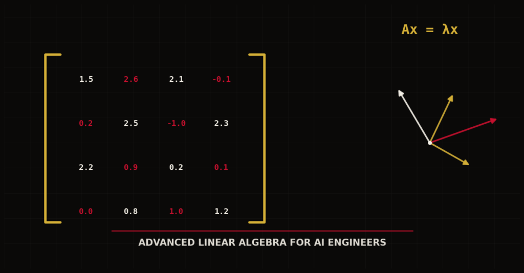
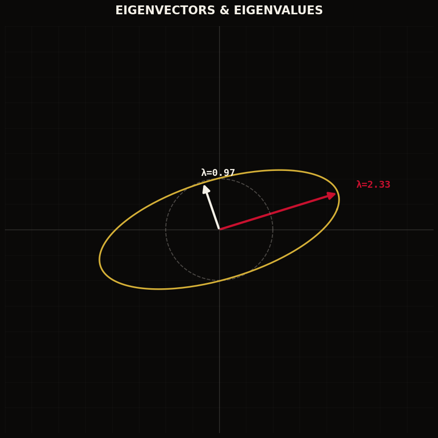
An eigenvector of a matrix is a direction that the matrix does not rotate — it only stretches or shrinks it. The scale factor is the corresponding eigenvalue. This single relationship — Av = λv — quietly powers PCA, spectral clustering, PageRank, and the stability analysis of recurrent networks.
Four Places Eigenvalues Quietly Run Production Systems
Principal Directions
The principal components of a dataset are exactly the eigenvectors of its covariance matrix.
RNN Training Dynamics
Eigenvalues of recurrent weight matrices >1 or <1 directly cause exploding or vanishing gradients.
PageRank & Graph Ranking
PageRank is literally the dominant eigenvector of a web-link transition matrix.
Spectral Clustering
Clusters emerge from the eigenvectors of a graph Laplacian, capturing non-linear structure.
NaN, the honest first answer is almost always “check the eigenvalue spectrum of your recurrent weight matrix” — not a framework bug.Matrix Decompositions
Decompositions break a matrix into simpler, structured pieces that are easier to compute with, more numerically stable, and often more interpretable. Four decompositions cover the overwhelming majority of production use cases.
| Decomposition | Structure | Primary Use Case |
|---|---|---|
| LU | A = L · U (lower × upper triangular) | Fast repeated solving of linear systems |
| QR | A = Q · R (orthogonal × upper triangular) | Stable least-squares regression, orthogonalization |
| Cholesky | A = L · Lᵀ (for positive-definite A) | Covariance matrices, Gaussian processes, fast sampling |
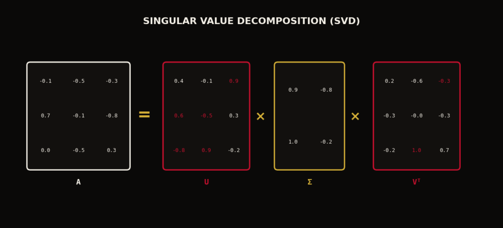
| SVD | A = U · Σ · Vᵀ | Dimensionality reduction, compression, recommender systems |
SVD in Production — Three Enterprise Use Cases
- Model compression — truncating a weight matrix’s SVD to its top-k singular values shrinks storage and inference cost while preserving most of the matrix’s information content.
- Recommender systems — classical matrix factorization (users × items) is SVD applied to a sparse interaction matrix to recover latent taste and item-quality dimensions.
- Noise reduction — dropping small singular values filters noise while preserving dominant structure, a technique used in signal processing pipelines across telecom infrastructure.
Principal Component Analysis in Practice
PCA finds the directions along which your data varies the most, and re-expresses the data in terms of those directions. Mechanically, it is nothing more than an eigendecomposition of a covariance matrix — everything before this chapter has been building toward this one, very practical algorithm.
- Standardize the data — center each feature to zero mean (and typically unit variance) so that features with large numeric ranges don’t dominate.
- Compute the covariance matrix — captures how every pair of features varies together.
- Eigendecompose the covariance matrix — the eigenvectors are the principal component directions; the eigenvalues are the variance explained along each one.
- Project the data — multiply the original data by the top-k eigenvectors to obtain a compressed, decorrelated representation.
from sklearn.decomposition import PCA

pca = PCA(n_components=50)               # compress to 50 dimensions
reduced = pca.fit_transform(features)     # shape: (n_samples, 50)
explained = pca.explained_variance_ratio_ # variance captured per component
Where PCA Earns Its Place in Production Pipelines
- Visualization — compressing high-dimensional embeddings to 2–3 dimensions for human inspection.
- Pre-training compression — reducing feature dimensionality before training to cut compute cost and mitigate the curse of dimensionality.
- Whitening — decorrelating features so downstream models converge faster and more stably.
- Anomaly detection — points that reconstruct poorly from their top principal components are strong anomaly candidates.
Linear Algebra Inside Neural Networks
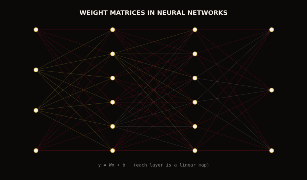
Strip away the diagrams and a neural network’s forward pass is a chain of matrix multiplications separated by element-wise nonlinearities. Backpropagation is the chain rule applied through that same chain, expressed as a sequence of Jacobian-vector products.
Backpropagation Is a Chain of Jacobians
For a loss L and a layer output y = Wx + b, the gradient with respect to the weights is computed via the chain rule as a matrix product involving the Jacobian of the loss with respect to y. In practice, deep learning frameworks compute this automatically via reverse-mode automatic differentiation — but reasoning about vanishing and exploding gradients requires understanding that each layer’s Jacobian gets multiplied into a long chain, and the eigenvalue spectrum of that chain determines whether gradients survive the trip back to early layers.
Convolutions Are Structured Matrix Multiplications
A convolution can be — and in some hardware implementations literally is — unrolled into a large sparse matrix multiplication (the “im2col” technique). Understanding this connection is what lets an engineer reason about the FLOP cost of a CNN layer using the exact same mental model as a dense layer.
Linear Algebra Inside Transformers
The transformer — the architecture behind every modern large language model — is, at its mathematical core, a small number of matrix operations applied repeatedly at scale. If you can read the attention formula fluently, you can read the architecture diagram of any modern LLM.
Query, Key, Value Projections
Three learned weight matrices project the input into three different subspaces for comparison.
QKᵀ — Similarity Matrix
A matrix multiplication produces a full pairwise similarity score between every token pair.
Softmax Normalization
Converts raw similarity scores into a probability distribution — the “attention weights.”
Weighted Sum via V
A final matrix multiplication blends value vectors according to the attention weights.
Why This Math Determines Real Engineering Constraints
The QKᵀ matrix has shape (sequence_length, sequence_length) — which is precisely why naive attention scales quadratically with context length, and why techniques like FlashAttention (which restructures the matrix computation to minimize memory movement rather than reduce FLOP count) became essential infrastructure rather than academic curiosities. Multi-head attention is simply this same computation performed in parallel across several lower-dimensional subspaces, then concatenated — a block-matrix operation.
Optimization: Gradients, Jacobians & Hessians
Training a model is an optimization problem, and every optimizer you’ve ever used — SGD, Momentum, Adam, RMSProp — is manipulating vectors and matrices derived from derivatives.
| Object | Definition | Role in Training |
|---|---|---|
| Gradient | Vector of first partial derivatives | Points in the direction of steepest loss increase; descent moves opposite it |
| Jacobian | Matrix of first partial derivatives of a vector-valued function | Propagates gradients backward through each layer |
| Hessian | Matrix of second partial derivatives | Describes loss curvature; used in second-order and trust-region methods |
Adam, the default optimizer for most modern training runs, maintains running estimates of the first and second moments of the gradient — effectively per-parameter vectors that adaptively rescale each update. Understanding Adam as “gradient descent with a per-parameter learned step size derived from gradient statistics” makes its hyperparameters (β₁, β₂, ε) far less mysterious.
Why Curvature Matters
The eigenvalues of the Hessian at a point describe the local curvature of the loss landscape in every direction. A saddle point — far more common than true local minima in high-dimensional loss landscapes — has a Hessian with both positive and negative eigenvalues. This is precisely why momentum-based optimizers, which retain velocity through flat and negatively-curved regions, generally outperform vanilla gradient descent on deep networks.
Enterprise-Scale: GPUs, TPUs & Distributed Compute
At enterprise scale, linear algebra stops being a whiteboard exercise and becomes a hardware-utilization problem. GPUs and TPUs are, quite literally, matrix-multiplication engines — understanding how your math maps onto that hardware is what separates a model that trains in days from one that trains in weeks.
Four Hardware-Level Concepts Every AI Engineer Should Know Cold
Specialized Matrix Units
Modern GPUs contain dedicated circuits optimized for small (e.g. 4×4) matrix multiply-accumulate operations at massive throughput.
FP16 / BF16 Matrix Ops
Running matrix multiplications in lower precision roughly doubles throughput and halves memory, with accuracy carefully preserved via master weights.
Sharded Weight Matrices
A single weight matrix too large for one device is split across GPUs, each computing a partial matrix product.
The Real Bottleneck
Modern training is frequently memory-bandwidth-bound, not compute-bound — matrix shape and data layout directly determine achievable throughput.
| Precision | Memory per Parameter | Relative Speed | Typical Use |
|---|---|---|---|
| FP32 | 4 bytes | 1x (baseline) | Reference / debugging precision |
| FP16 / BF16 | 2 bytes | ~2–3x | Standard mixed-precision training |
| INT8 | 1 byte | ~4x | Quantized inference at the edge |
Real-World Industry Applications
Telecom Network Optimization
Graph Laplacians — matrices built from a network’s connectivity structure — power anomaly detection across cell towers and backbone links; their eigenvalue spectrum reveals structural weaknesses and emerging congestion patterns long before a classical threshold-based alert would fire.
5G Signal Processing & Channel Estimation
MIMO channel estimation — a core 5G capability — is fundamentally a matrix estimation problem: recovering a channel matrix that describes how signals propagate between multiple antennas, then inverting or decomposing it to cancel interference and maximize throughput.
Recommendation Engines at Scale
Matrix factorization — an SVD variant applied to a sparse user-item interaction matrix — remains a foundational technique behind product and content recommendations, recovering latent taste dimensions that plain rule-based systems cannot capture.
Computer Vision & NLP Pipelines
Every convolutional feature extractor and every transformer-based language model ultimately reduces to the matrix operations covered in Chapters 9 and 10 — the industry difference is in how those operations are composed, regularized, and scaled, not in the underlying mathematics.
Fraud & Anomaly Detection
Covariance-matrix-based anomaly scoring — transactions that fall far from the principal subspace of “normal” behavior, as captured by PCA — remains one of the most robust, explainable first-line defenses in financial and telecom fraud systems, precisely because it’s grounded in interpretable linear algebra rather than an opaque black box.
Best Practices, Numerical Stability & Conclusion
Five Numerical-Stability Habits Every AI Engineer Should Build
- Never invert a matrix explicitly. Use
solve()instead ofinverse() @ b— it’s faster and dramatically more numerically stable. - Watch the condition number. A matrix with a huge condition number amplifies small input errors into large output errors — a frequent silent cause of training instability.
- Choose precision deliberately. Mixed precision is a default, not an afterthought, but master weights and loss scaling exist for a reason — understand why before disabling them.
- Vectorize instead of looping. Python loops over array elements throw away the entire performance advantage of matrix hardware; express operations as batched matrix algebra whenever possible.
- Regularize toward well-conditioned matrices. Weight decay, spectral normalization, and orthogonal initialization all exist to keep a network’s weight matrices numerically well-behaved throughout training.
Linear algebra has quietly become the shared vocabulary between AI research, systems engineering, and hardware design. The organizations pulling ahead in 2026 are the ones whose engineers move fluidly between all three — reading a paper’s equations, translating them into tensor shapes, and reasoning about how those shapes map onto GPU memory and FLOPs. That fluency compounds: every architecture you’ll encounter for the rest of your career is built from the same handful of operations covered in this guide.
Appendix A.1 — Formula Quick Reference
| Concept | Formula |
|---|---|
| Matrix multiplication | C = A · B |
| Eigen-relation | A v = λ v |
| SVD | A = U Σ Vᵀ |
| LoRA update | ΔW = B · A, rank r ≪ d |
| Attention | softmax(QKᵀ / √d) · V |
| Dense layer | y = φ(W·x + b) |
Appendix A.2 — Production Readiness Checklist
- Tensor shapes verified and logged at every major pipeline stage
- No explicit matrix inversion in the hot path — solvers used instead
- Condition number checked for ill-conditioned matrices before training
- Mixed-precision strategy chosen deliberately, not left on defaults blindly
- Low-rank / quantization compression evaluated before large-scale deployment
- Attention memory (KV-cache) budget estimated from matrix shapes before serving
- Weight matrix eigenvalue spectrum monitored for recurrent architectures
- Vectorized implementations used in place of manual loops
Go Build the Math Behind the Model 🧮
This guide is part of EDUNXT Tech Learning’s ongoing series translating core engineering concepts into practical, actionable frameworks for global founders and engineering teams.
Restart the Curriculum